by Divya Godayal

Asymptotic Analysis Explained with Pokémon: A Deep Dive into Complexity Analysis

by Sachin Malhotra and Divya Godayal

Let’s admit that we are either still stuck on the nuances of how to write a good algorithm or we dread the term itself.

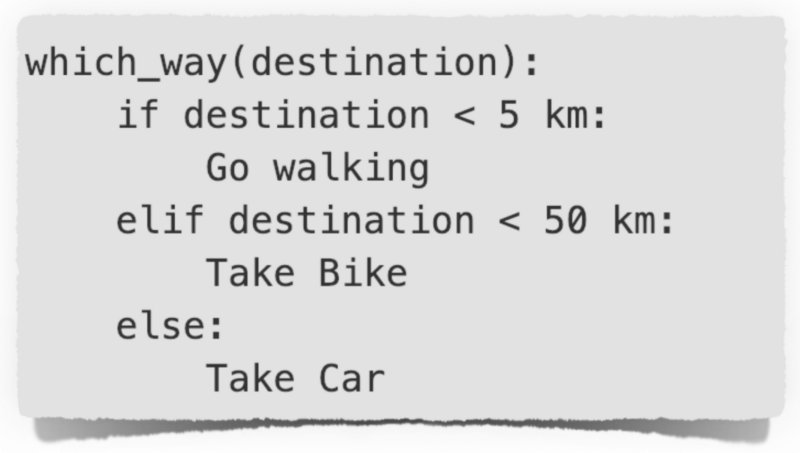
An algorithm is nothing fancy. It is just the method of doing something. For instance, let’s say Pikachu has to visit his friend tonight. He can do it in many different ways. What matters is which method he chooses.

The method he picks would determine the time taken for him to reach his friend. We deal with such scenarios on a daily basis. We might not think of every decision as an algorithmic decision, but it might be one.

Programmers need to make an informed choice every time. This matters even more when you are building a highly scalable and responsive application.

You are responsible for every piece of code you write, even if it doesn’t work. ?

Table of Contents ☞

• Why analyze an algorithm? 🧐
• Complexity and Asymptotic Behavior 🏋️‍♀️
• Degrees of Complexity ◎◉●○⦿
• Tools for Complexity Analysis 🛠
• Space Complexity 🌀
• The Time and Space trade-off 🎭
• Bubble Sort 🍸
• Insertion Sort 🃔🃕🂦
• Merge Sort 👫
• Recursion Tree Analysis 🌳
• Master Method Analysis 🤠🤙
• Binary Search 🧐 👉 👈

Why analyze an algorithm? 🧐

Algorithms are everywhere. Like literally, everywhere. In fact, to write this article we compiled a list of 1200 steps.

Don’t take that seriously now. I am kidding, of course! 🤭

What I mean is there is no escape from algorithms in any sphere of life. You better learn the art of picking the right one!

Let’s say our beloved Pokemon setup a championship. Whenever a pokemon wins a fight, its rank gets updated. To break the ties, the next fight is with the pokemon who shares the same score.

You are asked to build a website, which is quick at telling the next match. The coding ninja in you got excited and jumped on to it. You built a chic website, with cool graphics. You were initially told there are 50 Pokemon who would be part of the fight.

To find the next game of the winning pokemon, you decided to compare its score with the score of every pokemon in the championship, which is essentially linear search. And it worked like a charm!

But on the day of the first match, 1000 new pokemon (let’s just assume 😜) registered!! Aaaah, bummer. You didn’t see that coming, right?

Asymptotic Analysis is the evaluation of the performance of an algorithm in terms of just the input size (N), where N is very large. It gives you an idea of the limiting behavior of an application, and hence is very important to measure the performance of your code.

For example, if the number of pokemon taking part in the fight is N, then the asymptotic complexity of your linear search algorithm is O(N). If you don’t know what this notation is, fret not. We will address it soon.

In simple words, it’s like asking all the N pokemon what their rank is and then taking a decision. Imagine asking all 1000 pokemon. Tiring! right?

For a machine, O(N) might not be bad, but on a website where the focus is responsiveness and speed, it might not be the best choice.

The reason why 1000 new pokemon becomes a huge problem is because you didn’t think about the scalability aspect of the application from the get go and used a naive approach for solving the problem. Running into such scalability issues was just a matter of time.

Analysis of algorithms is like that, it’s always hanging around. But you only get serious about it when it’s really needed. And then you are just beating around the tail … uh oh, I mean the bush 😸

Analyzing an algorithm helps measures the efficiency of your program and it needs your attention from the moment you start thinking about a solution.

You could have just used a dictionary or a hash table to find all the pokemon with same rank and reduced the algorithmic time complexity to O(1). This is like going to just one manager pokemon who has the answer to your query.

A crazy reduction in time complexity, from O(N) to O(1). Analyzing an algorithm makes it possible to compare different approaches and decide on the best one.

What is N, by the way? 🤔

N defines the input. Here N are the number of Pokemons. For the purpose of algorithmic analysis, we consider N to be very large.

Complexity and Asymptotic Behavior 🏋️‍♀️

Let’s say Pikachu is on the lookout for a co-pokemon who has some kind of a special power. Pikachu starts by asking all the pokemon about their powers one by one. Such kind of an approach is known as linear search since it’s done linearly, one by one. But for our reference, let’s call it Pikachu’s Search.

1. Pikachu_Search(pokemon):              # List of pokemon
2.     for p in pokemon_list:           # No. of iterations -  N 
3.         if p has special power:  # Constant time operation
4.           return p               # Constant time operation
    
5.   return "No Pokemon Found"            # Constant time operation

In the above code snippet, pokemon_list is the list of all Pokemon participating in the championship. Hence, the size of this list is N.

Runtime Analysis for Pikachu’s Search:

1. Step 2is a for loop, thus the operations inside it will be repeated N times. Step 4is only executed if the condition in the step 3 is true. Once step 4is executed the loop breaks and result is returned.
2. If Step 3takes a constant amount of time, sayC1, then the total time taken in the for loop would be C1.N.
3. All the other operations are constant time operations not affected by the loop so we can take a cumulative constant for all of them as C2.

Total Runtime f(N) = C1.N + C2 , a function of N.

Let’s make it large. What if the value of N is very, very large. Do you think the constants would have any significance then?

In algorithmic analysis, an important idea is to chop off the less important part.

For example, if the run time for an algorithm is expressed as10N² + 2N + 5then asymptotically, only the higher order term N² is of significance. This makes comparison between algorithms much easier.

Degrees of Complexity ◎◉●○⦿

An algorithm shows different behaviors when exposed to different types of inputs. This brings us to the discussion of how we can define this behavior or the complexity of the algorithm. Since Pikachu’s search is still on, let’s see what’s going on with him.

1. Best Case ~ Pure Optimism. He got very lucky since the very first pokemon he approached had the special power Pikachu was looking for.
2. Worst Case ~ Pure Pessimism. He had to go visit all the pokemon and to his dismay, the very last pokemon had the super power which he wanted.
3. Average Case ~ Being Practical. Pikachu is a grown up Pokemon now. Experience has taught him a lot and he knows it’s all a matter of time and luck. He estimated high chances of finding the super Pokemon in the first 500 or so Pokemon that he visits and he was right.

Analyzing an algorithm could be done in the above mentioned three ways.

The best case complexity does not yield much. It acts as the lower bound for the complexity of an algorithm. If you go with it, you are just preparing yourself for the best. You have to be pretty lucky for your algorithm to hit the best case bounds anyways. In a practical sense, this doesn’t help much.

Always a good to know, the average case complexity is generally difficult to calculate because it needs you to analyze the performance of your algorithm on different variations of the input and hence not widely used.

Worst case complexity helps you prepare for the worst. In algorithms this kind of pessimism is considered good since it gives an upper bound on the complexity. Hence, you always know the limits of your algorithm!

Tools for Complexity Analysis 🛠

We saw earlier that the total runtime for Pikachu’s Search is f(N)= C1.N + C2 , a function of N. Let’s get to know more about the tools we have, to represent the running time, so as to make comparison among algorithms possible.

Big O 😮: Oh yes! It’s pronounced like that. Big — Oh ! It’s the upper bound on the complexity of an algorithm. Hence, it is used to denote the worst behavior of an algorithm.

Essentially, this denotes the maximum runtime for an algorithm no matter the input.

It is the most widely used notation because of its ease of analyzing an algorithm by learning about its worst behavior.

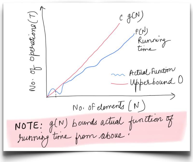
For Pikachu’s search, we can say f(N) or running time is bounded from above by C.g(N)for very large N, where is c is a constant and g(N) = N . Thus O(N)represents the asymptotic upper bound for Pikachu’s search.

Big Omega(Ω): Similar to Big O notation, the Ω notation is used to define an asymptotic lower bound on the performance of an algorithm. Hence, this is used for representing the best case scenarios.

The omega bound essentially means the minimum amount of time that our algorithm will take to execute, irrespective of the input.

This notation is not used often in practical scenarios, since studying the best behavior can’t be a correct measure for comparison.

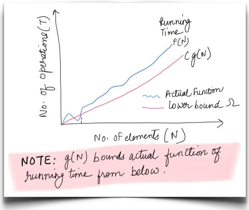
For Pikachu’s search, we can say f(N) or running time is bounded from below by C.g(N)for very large N, where is c is a constant and g(N) = 1. Thus Ω(1) represents the asymptotic lower bound for Pikachu’s Search.

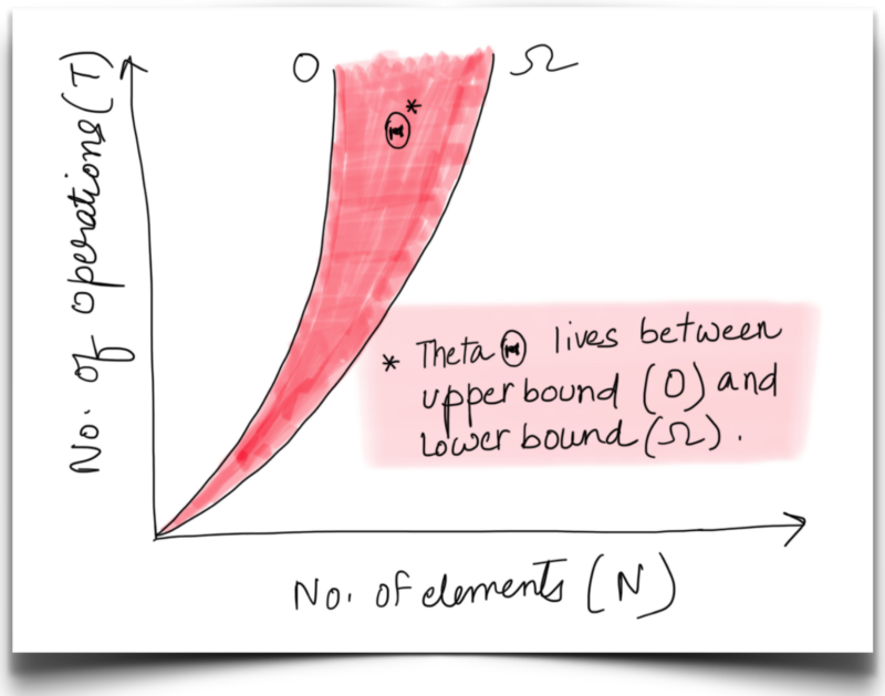
Big Theta(Θ): A tight bound on the behavior of an algorithm, this notation defines the upper and lower bounds for a function. This is called a tight bound because we fix the running time to within a constant factor above and below. Something like this:

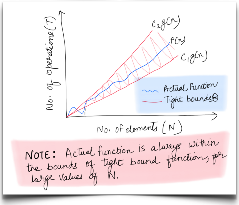
An algorithm might exhibit different best and worst case behaviors. When both are the same, we tend to use the theta notation. Otherwise, the best and worst cases are called out separately as:

(a) For worst case f(N) is bounded by function g(N) = N, for large values of N. Hence tight bound complexity would be denoted asΘ(N). This means the worst case run time for Pikachu’s search is at least C1​⋅N and at most C2⋅N.

(b) Similarly, its best case tight bound complexity is Θ(1).

Let’s consider one more example where f(N) = 10N² + 2N + 5, for this function the best and worst case complexities would be Ω(N²) and O(N²) respectively. Hence the average or the tight bound complexity would be Θ(N²).

Since worst case complexity acts as a better comparison metric, from now on we will be using Big-O for complexity analysis.

Space Complexity 🌀

We have been discussing about time complexity all this while. An important concept in complexity analysis is Space Complexity. As the name suggests, it means how much space or memory will the algorithm take in terms of N, where N is very large.

Whenever we compare different algorithms for solving a particular problem, we don’t just focus on the time complexities. Space complexity is also an important aspect for comparing different algorithms. Yes, it’s true that we have a lot of memory available these days and hence, space is something which can be compromised on. However, it is not something we should ignore all the time.

There’s an interesting conundrum that developers face all the time when coming up with solutions for programming problems. Let’s discuss a little bit about what it is.

The Time and Space trade-off 🎭

More often than not, you want to make your algorithm blazingly fast. Sometimes in doing so you end up compromising the space complexity.

However, sometimes we trade in some time to optimize on the space.

In practical applications, one thing or the other is compromised and this is famously referred to as the time-space tradeoff in the algorithmic analysis world.

Pikachu realized that he was searching for a pokemon every other day. This essentially means running Pikachu’s Search over and over again. Huh ! 😰 Naturally, he got so tired with the exhausting amount of work he had to put in everyday.

In order to help him out and speed up his search process, we decided to use a hash table. We can use the power type of a pokemon as the key in the hash table.

If we need to find the pokemon with a special power, the worst case complexity would be O(1), since hash table lookup is a constant time operation.

Without using this hash table, poor little Pikachu would have had to go visit every pokemon individually and ask about their powers. And repeatedly doing this is insane.

All it took was creating a hash table once and from then on use it for look-ups to bring down the overall runtime!

But that’s not it, as you saw it came with a cost of space. The hash table would need an entry for each Pokemon. Hence the space complexity would be O(N).

O(N) Time, O(1) Space —— Choose between — — O(1) Time, O(N) Space

This choice depends on the application needs. If we have a customer facing application, it should not be slow. The priority in such a situation would be making the application as responsive as possible no matter the amount of space used. However, if we’re really constrained by the space available to us, we have to give up on time to make up for that.

Choosing your algorithm wisely helps to optimize both time and space.

Time and Space complexity always go hand in hand. We need to do the math and go with the best approach. There is golden rule to help you decide which one to compromise on. Everything is application dependent.

That’s a lot of theoretical concepts to soak in. We know, even poor Pikachu has gotten a bit bored. But worry not, we will now put all these concepts into some practice and use them to analyze the complexity of some algorithms. This will help clarify the minute differences between the different kinds of complexities, the importance of big-Oh complexity, the time-space tradeoff and more.

To start with, Pikachu wants to analyze all the sorting techniques. Sorting all the Pokemons by their ranks helps him to keep the rank table organized.

Let’s check out the basic yet crucial sorting algorithms. The input array pk_rank to be sorted is of size N.

In case you are not familiar with any of the sorting algorithms mentioned below, we advice you to read about them before moving onto the following sections. The intention of the following examples is not to explain the different algorithms but to explain how you can derive their time and space complexity.

Bubble Sort 🍸

The bubble sort, one of the simplest of sorting algorithms repeatedly compares adjacent elements of an array and swaps them if they are out of order. The analogy is drawn from bubbles which rise to the top eventually. As elements of an array are sorted, they gradually bubble to their correct position in the array.

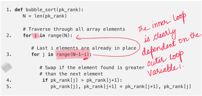
Time Complexity: Now that we have the algorithm in place, let’s get to analyzing its time and space complexity. We can clearly see from step 2 and 3 there is a nested loop structure in the algorithm. Also the range of the second for loop is N — 1 — i, which clearly indicates it is dependent on the previous loop.

if i = 0, second for loop would execute N-1 times
if i = 1, second for loop would execute N-2 times
if i = 2, second for loop would execute N-3 times
.
.
if i = N-1, second for loop would execute 0 times

Now we know the amount of time (iterations) our bubble sort algorithm takes at each step along the way. We mentioned before that there is a nested loop in the algorithm. For each value of the variable in the first loop, we know the amount of time taken in the second loop. All that remains now is to sum these up. Let’s do that.

S = N-1 + N-2 + N-3 + ... + 3 + 2 + 1
~ N * (N+1) / 2 
~ N² + N, ignoring all the coefficients

If you look at step 4and step 5, these are constant time operations. They don’t really add anything to the time complexity (or space complexity for that matter). That implies, we have N² + N iterations and in each iteration, we have constant time operations being performed.

Hence, the runtime complexity of bubble sort algorithm would be C.(N² + N) where C is a constant. Asymptotically we can say the worst case time complexity for Bubble Sort is O(N²).

Is this a good sorting algorithm? We haven’t looked at any other algorithms as such to compare with. However, let’s see how long it will take for this algorithm to sort a billion pokemon (reproduction, overpopulation, you get it 😛).

We leave the calculation up to you, but, it will take bubble sort approximately 31,709 years to sort a billion pokemon (assuming every instruction takes 1 ms to execute). Is Pikachu immortal or something 🤔

Space Complexity: Analyzing the space complexity is comparatively simpler as opposed to the time complexity for this algorithm. The bubble sort algorithm only performs one operation repeatedly. Swapping of numbers. In doing this, it doesn’t make use of any external memory. It just re-arranges the numbers in the original array and hence, the space complexity is constant, or O(1) or even Θ(1).

Insertion Sort 🃔🃕🂦

Do you like playing cards?

Well, even if you don’t, you should know that a good initial strategy in a lot of games is to arrange the cards in a specific order i.e. to sort the deck of cards. The idea for insertion sort is very similar to arranging the deck of cards.

Let’s say, you have a few cards sorted in ascending order. If you are given another card to be inserted at the right position so that the cards in your hand are still sorted. What will you do?

You would start from either the left or the right extreme of the cards in hand and compare the new card with every card in the deck and find the right spot.

Similarly, if more new cards are provided, you repeat the same process for each new card and keep the cards in your hand sorted.

Insertion sort works in the same manner. It starts from index 1 (array ordering starts at 0) and treats each element like a new card. Each of the new element can then placed at the correct position in the already sorted left subarray.

The important thing to note here is, given a new card (or an element in our case at an index j), all the cards in the hand (or all the elements before that index) are already sorted.

Let’s look at a formal algorithm for insertion sort followed by an animation that executes the algorithm on a test input.

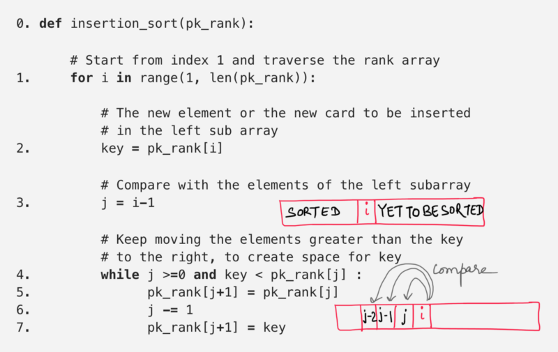
Time Complexity: From step 1 and 4there is a nested while structure within a for loop. The while loop runs j+1 times and j is clearly dependent on i. Let’s see how value of j changes with changing values of i.

if i = 1, then j = 0 hence while loop would execute 1 times
if i = 2, then j = 1 hence while loop would execute 2 times
if i = 3, then j = 2 hence while loop would execute 3 times
.
.
if i = N-1, then j = N-2 hence while loop would execute N-1 times

Now we know the amount of time (iterations) our insertion sort algorithm takes at each step along the way. Total time is:

S = 1 + 2 + 3 + .... + N-2 + N-1
~ N * (N+1) / 2 
~ N² + N, ignoring all the coefficients

Step 2 through 7 are constant time operations. They don’t really add anything to the time complexity (or space complexity for that matter). That implies, we have N² + N iterations and in each iteration, we have constant time operations being performed.

Hence, the runtime complexity of the insertion sort algorithm would be C.(N² + N) where C is a constant. Asymptotically, we can say the worst case time complexity for Insertion Sort is same as that of bubble sort i.e. O(N²).

Space Complexity: Analyzing the space complexity is comparatively simpler as opposed to the time complexity for this algorithm. The insert sort algorithm only re-arranges the numbers in the original array. In doing this, it doesn’t make use of any external memory at all. Hence, the space complexity is constant, or O(1) or even Θ(1).

Note: Comparing algorithms on the basis of asymptotic complexity is easy and fast. Also on a higher level it’s a good measure. But from practical aspects if two algorithms have same complexity, it doesn’t necessarily mean they have same performance in practical scenarios.

When calculating the asymptotic complexity of an algorithm, we ignore all the constant factors and the lower order terms.

But these ignored values eventually do add to the execution time of an algorithm.

Insertion sort is much faster than bubble sort when the array is almost sorted. For each pass through the array, bubble sort must go till the end of the array and compare the adjacent pairs, insertion sort on the other hand, would bail early if it finds that the array is sorted. Try executing the two algorithms on a sorted array and look at the number of iterations it takes each of them to finish execution.

Thus, whenever you are finding the best algorithm for your application, it needs to be analyzed from a lot of different aspects. Asymptotic analysis definitely helps to weed out slower algorithms, but observation and deeper insights help to find the best suited algorithm for your application.

Merge Sort 👫

So far we’ve analyzed two of the most basic sorting algorithms. These are introductory sorting algorithms but are not the ones generally used in practice due to their high asymptotic complexity.

Let’s move on to a faster, more practical sorting algorithm. The merge sort algorithm deviates from the nested loop structured sorting that we have seen in the previous two algorithms and adopts a completely new paradigm that we will be discussing below.

The Merge Sort algorithm is based on something known as the Divide and Conquer programming paradigm. This programming paradigm is based on a very simple idea and this finds utility in a lot of different algorithms out there including merge sort. Divide and Conquer is divided into three basic steps:

Divide: Break a big problem into smaller sub-problems.
Conquer: Optimally solve the smaller sub-problems
Combine: Finally, combine the results of the sub-problems to find the solution for the original big problem.

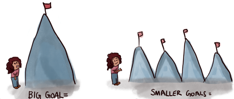
Let’s look at a brief overview of how the merge sort algorithm makes use of the divide and conquer paradigm.

1. Divide ~ The first step in the process is to divide the given array into two, equal-sized smaller sub-arrays. This helps since now we have 2 smaller arrays to sort, each with half the original number of elements.
2. Conquer ~ The next step is to sort the smaller arrays. This part is referred to as the conquer step since we are solving the sub-problems optimally.
3. Combine ~ Finally, we are presented with two sorted halves of the original array and we have to combine them optimally such that we get a single sorted array. This is the combine step of the paradigm explained above.

But wait. Is this it?

Given an array of 1000 elements if we divide it into 2 equal halves of 500 each, we still have a lot of elements to sort in an array (or sub-array).

Shouldn’t we divide the two halves further into 4 to get even shorter subarrays?

Yes! Indeed we should!

We recursively divide the array into smaller halves and sort and merge the smaller halves to get the original array back.

This essentially means we divide e.g. an array of size 1000 into 2 halves of 500 each. Then we further split these two halves into 4 portions of 250 each and so on. Don’t worry if you’re not able to contemplate all of this intuitively in terms of complexity analysis. We will get to that very soon.

Let’s have a look at the algorithm for merge-sort. The algorithm is divided into two functions, one which recursively sorts the two equal halves of a given array and another one which merges the two sorted halves together.

We will first analyze the complexity of the merge function and then get to analyzing the merge_sort function.

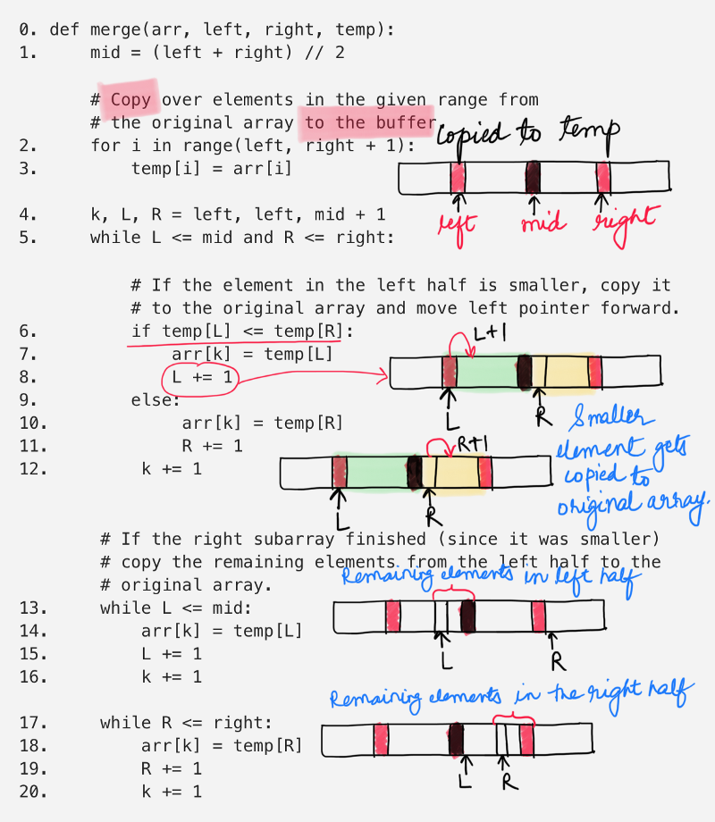
The above function simply takes in two sorted halves of the array and merges them together into a single, sorted half. The two halves are defined using indices. The left half is from [left, mid] and the right half is from [mid + 1, right].

step 2-3 copies the elements over from the original array to a temporary buffer and we use this buffer for merging purposes. The sorted elements are copied back to the original array. Since we iterate over a certain portion of the array, the time complexity for this operation is O(N) considering there are N elements in the array.

step 5 is a while loop which iterates over the shorter one of the two subarrays. This while loop and the ones that come after, in step 13 and step 14 cover all the elements of the two subarrays. So, their combined time complexity is O(N).

This means that the merging step is a linear time algorithm.

The overall complexity of the merge sort is decided by the number of times the merge function is called.

Let’s move on and look at the original merge_sort function. It’s extremely simple.

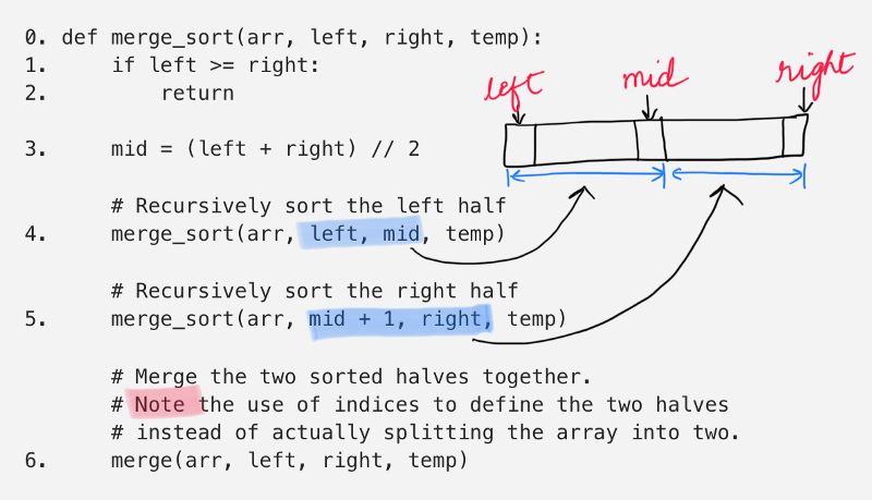
step 4 calls the merge_sort function on the left half of the array.

step 5 calls the merge_sort function on the right half of the array.

and then the step 6 finally calls the merge function to combine the two halves.

Uh. A function calling itself? 🤨🤨

How does one calculate it’s complexity?

Till now we have discussed analysis of loops. Many algorithms, however, like Merge Sort are recursive in nature. When we analyze them, we get a recurrence relation for time complexity. We get running time on an input of size N as a function of N and the running time on inputs of smaller sizes.

Primarily, there are two important ways of analyzing the complexity of a recurrence relation:

1. Using a Recursion Tree and
2. Using the Master Method.

Recursion Tree Analysis 🌳

This is the most intuitive way for analyzing the complexity of recurrence relations. Essentially, we can visualize a recurrence relation in the form of a recursion tree.

The visualization helps to know the amount of work done by the algorithm at each step (read level) along the way and summing up the work done at each level tells us the overall complexity of the algorithm.

Before we look at the recursion tree for the Merge Sort algorithm, let’s first look at the recurrence relation for it.

T(N) = 2T(N / 2) + O(N)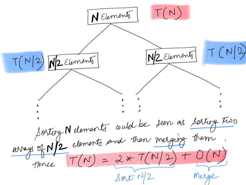

Let T(N) represent the amount of work done (or the time taken to) sort an array consisting of N elements. The above relation states that the overall time taken is equal to the time taken to sort the two halves of the array + the time taken to merge the two halves. We have already seen the time taken to merge the two halves before and that is O(N).

We can write the recurrence relation as follows:

T(N) = 2T(N / 2) + O(N)
T(N / 2) = 2T(N / 4) + O(N / 2)
T(N / 4) = 2T(N / 8) + O(N / 4)
...

It’s much easier to visualize this in the form of a tree. Each node in the tree would consist of two branches since we have two different subproblems given a single problem. Let’s look at the recursion tree for merge sort.

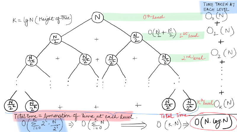
Each node in the tree represents a subproblem and the value at each node represents the amount of work spent at each subproblem. The root node represents the original problem.

In our recursion tree, every non-leaf node has 2 children, representing the number of subproblems it is splitting into. We have seen from the algorithm for Merge Sort that at each step of the recursion, the given array is divided into two equal halves.

So, there are two important things we need to figure out in order to analyze the complexity of the merge sort algorithm.

1. We need to know the amount of work done at each level in the tree and
2. We need to know the total number of levels in the tree, or, as it is more commonly called, the height of the tree.

First, we will calculate the height of our recursion tree. We can see from the recursion tree above that every non-leaf node splits into two nodes. Hence, what we have above is a complete binary tree.

Intuitively, we will go on splitting the array until there is a single element left in a subarray, at which point we don’t need any sorting (this is the base case) and we simply return.

At the first level in our binary recursion tree, there is a single subproblem consisting of N elements. The next level in the tree consists of 2 subproblems (sub-arrays to be sorted) with N / 2 elements each.

Right now, we are not really concerned with the number of subproblems. We just want to know the size of each subproblem since we can see that all the subproblems on a particular level of the tree are of the same size.

At Level 0 we have subproblem(s) each consisting of N    elements
At Level 1 we have subproblem(s) each consisting of N/2  elements
At Level 2 we have subproblem(s) each consisting of N/4  elements
At Level 3 we have subproblem(s) each consisting of N/8  elements
At Level 4 we have subproblem(s) each consisting of N/16 elements
.
.
.
At Level X we have subproblem(s) each consisting of 1 element.

The number of elements seem to be reducing in powers of 2. From the pattern above, it seems that:

N = 2^X 
X = log_2(N)

This means, the height of our tree is log_2(N) (log base 2 of N). Now let’s look at the amount of work done by the algorithm at each step.

T(N) is defined as the amount of work required to be put in for sorting an array of N elements. We looked at the recurrence relation for this earlier on and it was:

T(N) = 2T(N / 2) + O(N)

This implies, the amount of work done at the first level in the tree is O(N) and rest of the work is done at the next level. This is due to the recursion call in the form of 2T(N / 2) . At the next level, as we can see from the figure above, the amount of work done is 2 * O(N / 2) = O(N). Similarly, the amount of work done at the third level os 4 * O(N / 4) = O(N).

Surprisingly, the algorithm has to perform the same amount of work on each level and that work amounts to O(N) which is the time consumed by the merge procedure. Thus, the number of levels will define the overall time complexity.

As we calculated earlier, the number of levels in our recursion tree are log(N) and hence, the time complexity for Merge Sort is O(Nlog(N)).

Yay! We learnt a new methodology for asymptotic analysis in the form of recursion trees. It’s a fun way to build an intuition about the complexity of any recurrence relation. It may not always be feasible to draw out the complete recursion tree, but it definitely helps build an understanding.

Master Method Analysis 🤠🤙

We’ve looked at the recursion tree based method for asymptotic analysis of recurrences. However, as mentioned before, it might not be feasible to draw out the recursion tree every time for calculating the complexity.

The merge sort recursion breaks a given problem (array) into two smaller sub-problems (subarrays). What if we get an algorithm where a problem is divided into say, 100 subproblems? We won’t be able to draw out the recursion tree for analysis.

Thus, we need a more direct way for analyzing the complexity of a recurrence relation. We need a method which doesn’t require us to actually draw the recursion tree but one which builds on the same concepts as the recursion tree.

This is where the Master Method comes into the picture. This method is based on the recursion tree method. There are three different scenarios that are covered under the master method which essentially cover most of the recurrence relations. Before looking at these cases, however, let’s look at the recursion tree for the following general recursion relation:

T(n) = a T(n / b) + f(n)

• n is the size of the problem.
• a is the number of subproblems in the recursion.
• n / b is the size of each subproblem. (Here it is assumed that all subproblems are essentially the same size.)
• f(n)is the cost of the work done outside the recursive calls, which includes the cost of dividing the problem into smaller subproblems and the cost of merging the solutions to the subproblems.

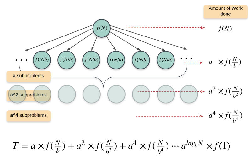
The two most important things to know for us to understand the master method are the amount of work done by the algorithm at the root and the amount of work done at the leaves.

The work done at the root is simply f(n). The amount of work done at the leaves is dependent upon the height of the tree.

The height of this tree would be log_b(n) i.e log base b of n. This follows from the recursion tree we saw for merge sort. b in case of merge sort is 2. The number of nodes at any level, l are a^l and so, the number of leaf nodes at the last level would be:

a^{log_b(n)} = n ^ log_b(a) nodes.

Since the amount of work done on each subproblem at the final level is Θ(1), the total amount of work done at the leaf nodes is n ^ log_b(a).

If you focus on the generic recurrence relation above, you will notice that there are two main competing forces at play:

1. The Division step ~ the 𝑎𝑇(𝑛/𝑏) term is desperately trying to reproduce, multiplying smaller and smaller copies of itself.
2. The Conquer step ~ the 𝑓(𝑛) term represents merging since it is desperately trying to collapse these mini-portions together.

The two forces are trying to oppose the other one and in doing so, they want to control the total amount of work done by the algorithm and hence the overall time complexity.

Who will win ?

Case 1 (Divide Step Wins)

If f(n) = Θ(n^c) such that c < log_b(a), then T(n) = Θ(n^log_b(a). f(n) is the amount of work done at the root of the tree and n ^ log_b(a) is the amount of work done at the leaves.

If the work done at leaves is polynomially more, then leaves are the dominant part, and our result becomes the work done at leaves.

e.g. T(n) = 8 T(n / 2) + 1000 n^2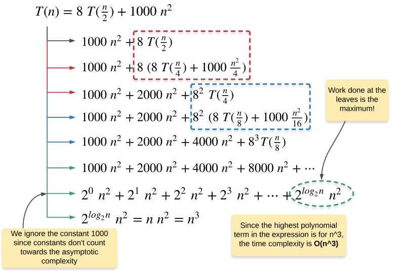

If we fit this recurrence relation in the Master method, we get:

a = 8, b = 2, and f(n) = O(n^2)
Hence, c = 2 and log_b(a) = log_2(8) = 3
Clearly, 2 < 3 and this fits in the Case 1 for Master method. This implies, the amount of work done at the leaves of the tree is asymptotically higher than the work done at the root. Hence, the complexity of this recurrence relation is Θ(n^log_2(8)) = Θ(n^3).

Case 2 (Conquer Step Wins)

If f(n) = Θ(n^c) such that c > log_b(a), then T(n) = Θ(f(n)). If work done at root is asymptotically more, then our final complexity becomes work done at root.

We are not concerned with the amount of work done at the lower levels here, since the largest polynomial term dependent on n is the one that controls the complexity of the algorithm. Hence, the work done on all the lower levels can be safely ignored.

e.g. T(n) = 2 T(n / 2) + n^2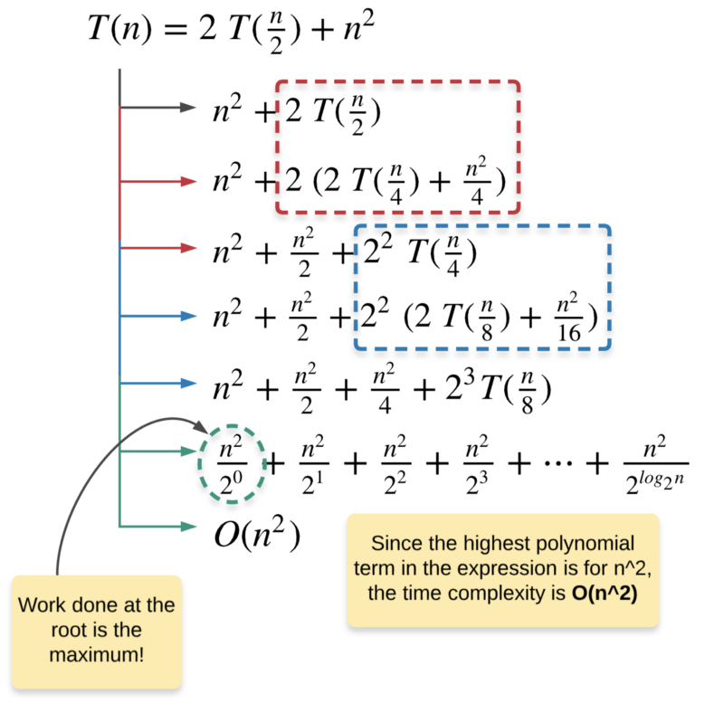

If we fit this recurrence relation in the Master method, we get:

a = 2, b = 2, and f(n) = O(n^2)
Hence, c = 2 and log_b(a) = log_2(2) = 1
Clearly, 2 > 1 and hence this fits the Case 2 of the Master method where majority of the work is done at the root of the recursion tree and that is why Θ(f(n)) controls the complexity of the algorithm. Thus, the time complexity of this recurrence relation is Θ(n^2).

Case 3 [It’s a tie!]

If f(n) = Θ(n^c) such that c = log_b(a), then T(n) = Θ(n^c log(n)).The final case is when there’s a tie amongst the work done at the leaves and the work done at the root of the tree.

In this case, both the conquer and the divide steps are equally dominant and hence, the total amount of work done is equal to the the work done at any level * height of the tree.

e.g. T(n) = 2T(n / 2) + O(n)

Yes! This is the complexity of the Merge Sort algorithm. If we fit the recurrence relation for merge sort in the Master method, we get:

a = 2, b = 2, and f(n) = O(n^1)
Hence, c = 1 = log_2(2)
This fits the criterion for the Case 3 described above. The amount of work done is same on all the levels as can be verified from the figure above. Thus, the time complexity is the work done at any level * the total number of levels (or the height of the tree).

We have analyzed the time complexity of the Merge Sort algorithm using two different ways namely the Recursion Tree and the Master Method. We had to use these different techniques since the merge sort algorithm is a recursive algorithm and the classical asymptotic analysis approaches we had seen earlier for loops were of no use here.

Space Complexity: As for the space complexity, we don’t have to use any complicated techniques and hence, the analysis is much simpler. One main space occupying data structure in the Merge Sort algorithm is the temp buffer array that is used during the merge procedure.

This array is initialized once and the size of this array is N. Another data structure that occupies space is the recursion stack. Essentially, the total number of recursive calls determine the size of the recursion stack. As we’ve seen in the recursion tree representation, the number of calls made by merge sort is essentially the height of the recursion tree.

The height of the recursion tree was log_2(N) and hence, the size of the recursion stack will also be log_2(N) at max.

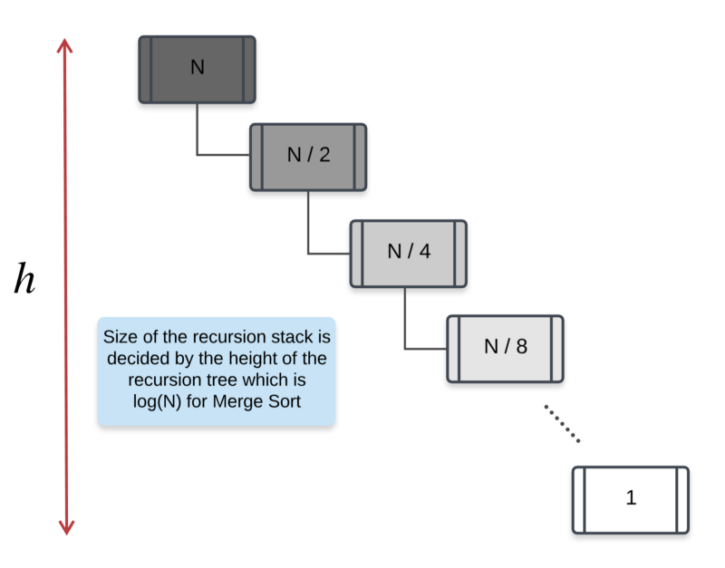
Hence, the total space complexity for merge sort would be N + log_2(N) = O(N).

Binary Search 🧐 👉 👈

Remember our friend Pikachu and his search for a Pokemon of a specific power. Poor little Pikachu had a 1000 Pokemon at his disposal and he had to find the one Pokemon with a specific power. Yeah, Pikachu is very choosy about his opponents.

His requirements keep on changing day in and day out and he certainly cannot go and check with each and every Pokemon, every time his requirements change i.e. he cannot perform a Linear Search through the list of Pokemon to find the one he is looking for.

We mentioned earlier the use of a Hash Table to store the Pokemon using their unique power value as the key and the Pokemon itself as the value. This would bring down the search complexity to O(1) i.e. constant time.

However, this makes use of additional space which raises the space complexity of the search operation to O(N) considering there are N Pokemon available. N in this case would be 1000. What if Pikachu didn’t have all this extra space available and he still wanted to speed up the search process?

Yes! Certainly Pikachu can make use of his profound knowledge about sorting algorithms to come up with a search strategy which would be faster than the slow Linear search.

Pikachu decided to ask his good friend Deoxys for help. Deoxys, being the fastest Pokemon out there, helps Pikachu sort the list of Pokemon according to their power.

Instead of relying on the traditional sorting algorithms, Deoxys makes use of the Quick Sort algorithm (of course he does!) for sorting the Pokemon.

In doing so, he doesn’t make use of any additional space and the time taken for sorting the N Pokemon is the same as that of the Merge Sort algorithm. So, Pikachu is happy with his friend helping him out at the time of need.

Pikachu, being extremely smart, comes up with a search strategy which makes use of the sorted nature of the list of Pokemon. This new strategy /algorithm is known as the Binary Search algorithm. (Note: Sorting is a precondition for running binary search, once the list is sorted Pikachu can run binary search as many times as he wants on this sorted list).

Let’s have a look at the code for this algorithm and then analyze its complexity.

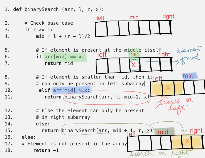
Clearly, the algorithm is recursive in nature. Let’s see if we can use our newly learnt tricks to analyze the time complexity for the binary search algorithm. The two variables l and r essentially define the portion of the array in which we have to search for the given element, x.

If we look at the algorithm, all it’s really doing is dividing the search portion of the input array into half. Other than making a recursive call based on a certain condition, it doesn’t really do anything. So, let’s quickly look at the recurrence relation for the binary search algorithm.

T(n) = T(n / 2) + O(1)

That seems like a pretty simple recurrence relation to analyze. First let’s try and analyze the recursion tree and draw the complexity from there and then we will look at the Master theorem and see which of the three cases fits this recursion.

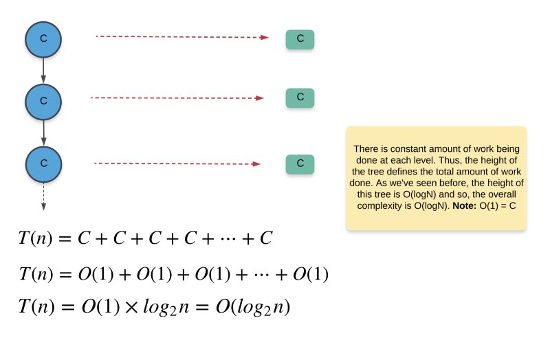
Whoa! This binary search algorithm is super fast. It’s much faster than linear search. What this implies for our cute little friend Pikachu is that for 1000 Pokemon, he would simply have to go and “ask” 10 of them at max to find the one special pokemon he is looking for (how? 🤓).

Now let’s see how the more “formulaic” way of approach recursive complexity analysis i.e. the Master method help us in this case. The generic master method recursive relation is

T(n) = a T(n / b) + f(n)

and for our binary search algorithm we have

T(n) = T(n / 2) + O(1)
f(n) = O(n^0), hence c = 0
a = 1
b = 2
c = 0

There are 3 different cases for the master theorem and c ? log_b(a) decides which of the three cases get’s used for a particular analysis. In our case, 0 < log_2(1) i.e. 0 = 0. This implies that our binary search algorithm fits the case-3 of the master theorem, therefore T(n) = Θ(n^0 log(n)) = Θ(log(n)

How to choose the best algorithm? 🤨

In this article we introduced the idea of complexity analysis which is an important part of algorithm design and development. We saw why analyzing an algorithm’s complexity is important and how it directly affects our scalability decisions. We even saw some great techniques for analyzing this complexity efficiently and correctly so as to make informed decisions in a timely manner. The question arises, however,

Given all that I know about the time and space complexities of two algorithms, how do I choose which one to finally go with? Is there a golden rule?

The answer to this question, unfortunately, is No!

There’s no golden rule to help you decide which algorithm to go with. It totally depends on a lot of external factors. Let’s try and look at a few of these scenarios that you might find yourself in and also look at the kind of decisions you would want to make.

No constraint on the space!

Well, if you have two algorithms A and B and you want to decide which one to use, apart from the time complexity, the space complexity also becomes an important factor.

However, given that space is not an issue that you are concerned with, it’s best to go with the algorithm that has the capability to reduce the time complexity even further given more space.

For example, Counting Sort is a linear time sorting algorithm but it’s heavily dependent upon the amount of space available. Precisely, the range of numbers that it can deal with depends on the amount of space available. Given unlimited space, you’re better off using the counting sort algorithm for sorting a huge range of numbers.

Sub-second latency requirement and limited space available

If you find yourself in such a scenario, then it becomes really important to deeply understand the performance of the algorithm on a lot of varying inputs especially the kind of inputs you expect the algorithm to work with in your application.

For example, we have two sorting algorithms: Bubble sort and Insertion sort, and you want to decide amongst them which one to use for sorting a list of users based on their age. You analyzed the kind of input expected and you found the input array to be almost sorted. In such a scenario, it’s best to use Insertion sort over Bubble sort due to its inherent ability to deal amazingly well with almost sorted inputs.

Wait, why would anyone use Bubble or Insertion sort in real world scenarios?

If you think that these algorithms are just for educational purposes and are not used in any real world scenarios, you’re not alone! However, this couldn’t be further away from truth. I’m sure you’ve all used the sort() functionality in Python sometime in your career.

Well, if you’ve used it and marveled at its performance, you’ve used a hybrid algorithm based on Insertion Sort and Merge Sort called the Tim Sort algorithm. To read more about it, head over here:

Timsort — the fastest sorting algorithm you’ve never heard of
Timsort: A very fast , O(n log n), stable sorting algorithm built for the real world — not constructed in academia…skerritt.blog

It’s true that insertion sort might not be useful for very large inputs as we’ve al seen from its polynomial time complexity. However, it’s inherent ability to quickly sort almost sorted range of numbers is what makes it so special and that’s precisely the reason it’s used in the Timsort algorithm.

In short, you won’t ever have a clear black and white division between the algorithms you are struggling to choose from. You have to analyze all the properties of the algorithms, including their time and space complexity. You have to consider the size of inputs you are expecting your algorithm to work with and any other constraints that might exist. Considering all these factors, you have to make an informed decision!

If you had a fun time understanding the intricacies of complexity analysis and also playing around with our friend Pikachu, do remember to destroy that like button and spread some love. ❣️

If you want more programming problems with detailed complexity analysis, head over to our kitchen! 🍩

Analyzing an algorithm is an important part of any developer’s skill set and if you feel there are other’s who might benefit from this article, then do share it as much as possible!