Graph Neural Networks are getting more and more popular and are being used extensively in a wide variety of projects.
In this article, I help you get started and understand how graph neural networks work while also trying to address the question "why" at each stage.
Finally we will also take a look at implementing some of the methods we talk about in this article in code.
And don't worry – you won't need to know very much math to understand these concepts and learn how to apply them.
What is a graph?
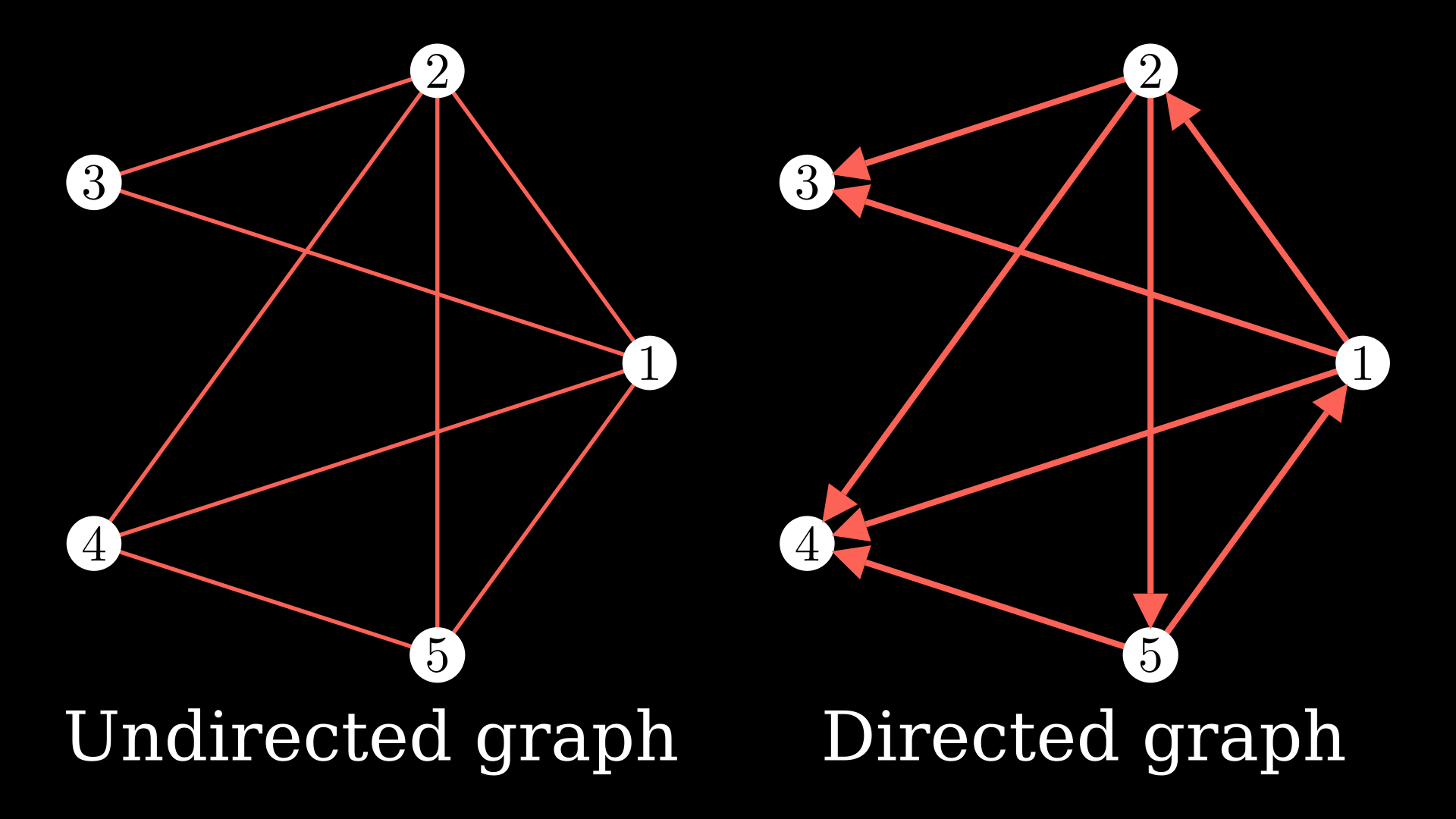
Put quite simply, a graph is a collection of nodes and the edges between the nodes. In the below diagram, the white circles represent the nodes, and they are connected with edges, the red colored lines.
You could continue adding nodes and edges to the graph. You could also add directions to the edges which would make it a directed graph.
Something quite handy is the adjacency matrix which is a way to express the graph. The values of this matrix \(A_{ij}\) are defined as:
\[A_{ij} = \left\{\begin{array}{ c l }1 & \quad \textrm{if there exists an edge } j \rightarrow i \\ 0 & \quad \textrm{if no edge exists} \end{array} \right. \]
Another way to represent the adjacency matrix is simply flipping the direction so in the same equation \(A_{ij}\) will be 1 if there is an edge \(i \rightarrow j\) instead.
The later representation is in fact what I studied in school. But often in Machine Learning papers, you will find the first notation used – so for this article we will stick to the first representation.
There are a lot interesting things you might notice from the adjacency matrix. First of all, you might notice that if the graph is undirected, you essentially end up with a symmetric matrix and more interesting properties, especially with the eigen values of this matrix.
One such interpretation which would be helpful in the context is taking powers of the matrix \((A^n)_{ij}\) gives us the number of (directed or undirected) walks of length \(n\) between nodes \(i\) and \(j\).
Why work with data in Graphs?
Well graphs are used in all kinds of common scenarios, and they have many possible applications.
Probably the most common application of representing data with graphs is using molecular graphs to represent chemical structures. These have helped predict bond lengths, charges, and new molecules.
With molecular graphs, you can use Machine Learning to predict if a molecule is a potent drug.
For example, you could train a graph neural network to predict if a molecule will inhibit certain bacteria and train it on a variety of compounds you know the results for.
Then you could essentially apply your model to any molecule and end up discovering that a previously overlooked molecule would in fact work as an excellent antibiotic. This is how Stokes et al. in their paper (2020) predicted a new antibiotic called Halicin.
Another interesting paper by DeepMind (ETA Prediction with Graph Neural Networks in Google Maps, 2021) modeled transportation maps as graphs and ran a graph neural network to improve the accuracy of ETAs by up to 50% in Google Maps.
In this paper they partition travel routes into super segments which model a part of the route. This gave them a graph structure to operate over on which they run a graph neural network.
There have been other interesting papers that represent naturally occurring data as graphs (social networks, electrical circuits, Feynman diagrams and more) that made significant discoveries as well.
And if you think abut it, a standard neural network can be represented as a graph too 🤯.
What can we do with Graph Neural Networks?
Let's first start with what we might want to do with our graph neural network before understanding how we would do that.
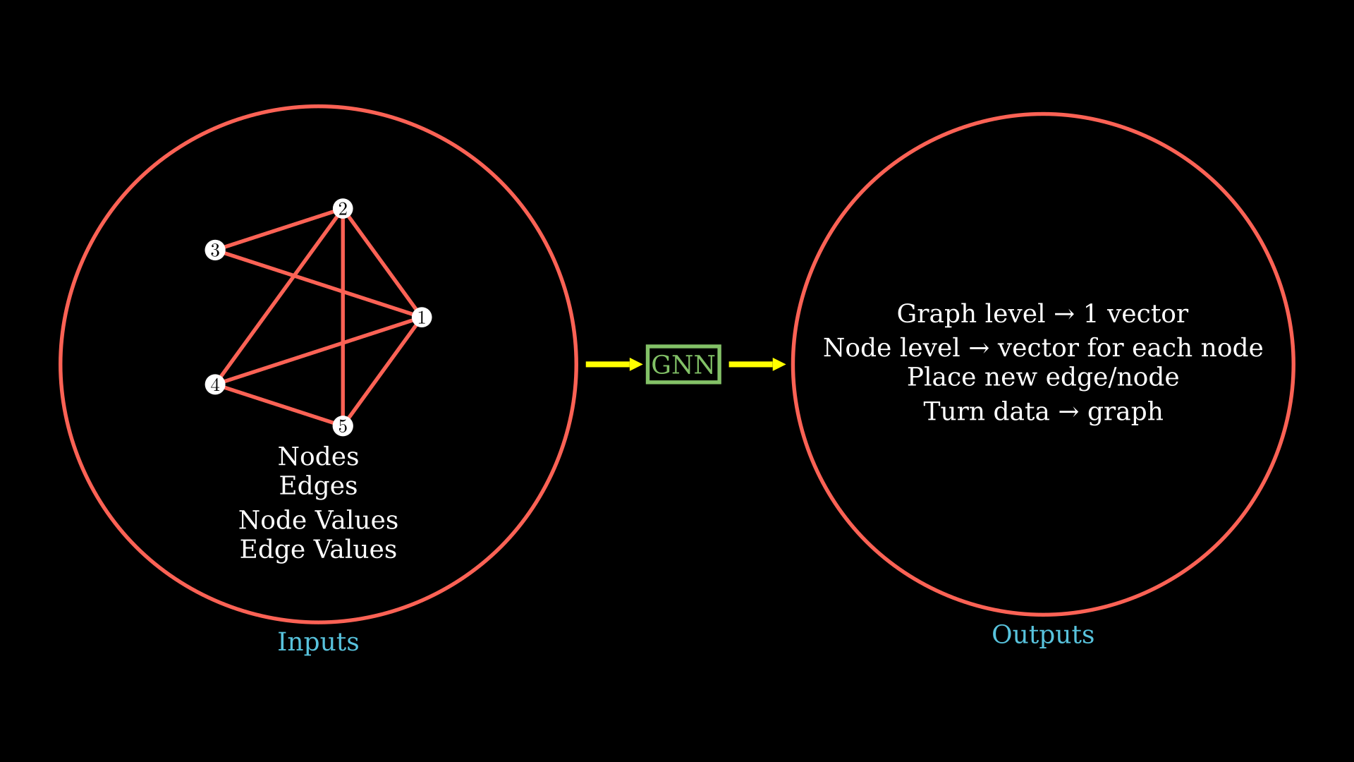
One kind of output we might want from our graph neural network is on the entire graph level, to have a single output vector. You could relate this kind of output with the ETA prediction or predicting binding energy from a molecular structure from the examples we talked about.
Another kind of output you might want is the node or edge level predictions and end up with a vector for each node or edge. You could relate this with an example where you need to rank every node in the prediction or probably predict the bond angle for all bonds given the molecular structure.
You might also be interested in answering the question "Where should I place a new edge or a node" or predict where an edge or a node might appear. We could not only get that prediction from the graph, but then we could also turn some other data into a graph.
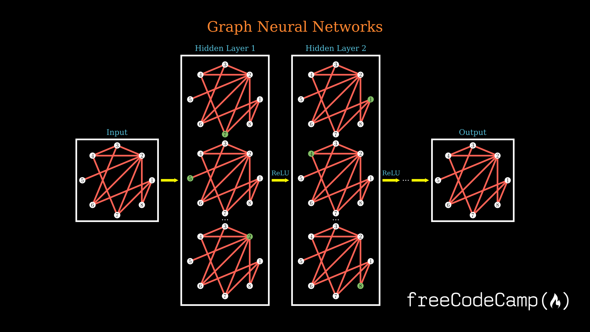
As you might have guessed with the graph neural network, we first want to generate an output graph or latents from which we would then be able to work on this wide variety of standard tasks.
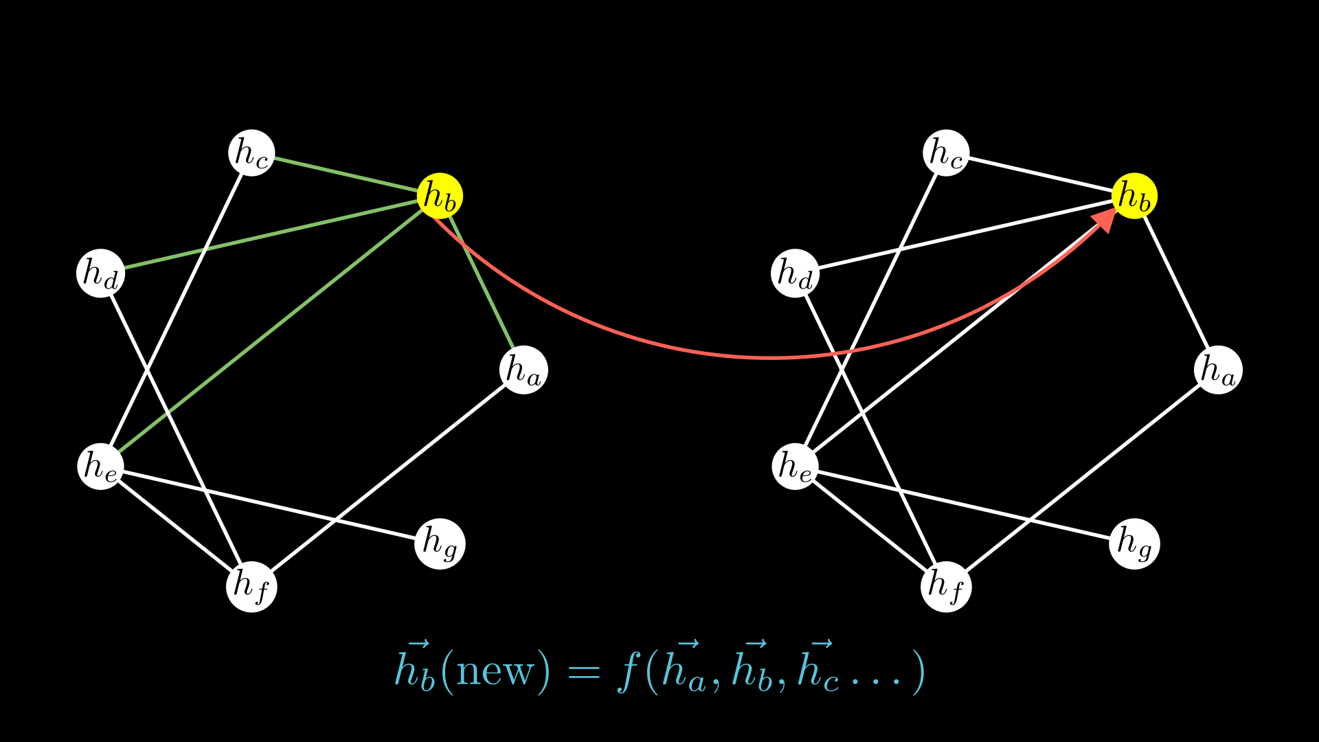
So essentially what we need to do from the latent graph (features for each node represented as \(\vec{h_i}\)) for the graph level predictions is:
- first figure out some way to aggregate all the vectors (like simply summing), and
- then create some function to get the predictions:
\[\vec{Z_G} = f(\sum_i \vec{h_i})\]
And now it is quite simple to show on a high level what we need to do from the latents to get our outputs.
For node level outputs we would just have one node vector passed into our function and get the predictions for that node:
\[\vec{Z_i} = f(\vec{h_i})\]
The problem with variable sized inputs
Now that we know what we can do with the graph neural networks and why you might want to represent your data in graphs, let's see how we would go about training on graph data.
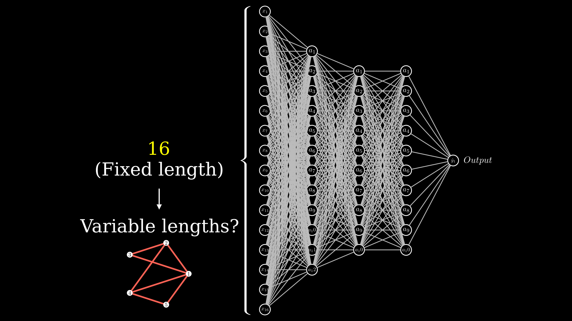
But first off, we have a problem on our hands: graphs are essentially variable size inputs. In a standard neural network, as shown in the figure below, the input layer (shown in the figure as \(x_i\)) has a fixed number of neurons. In this network you cannot suddenly apply the network to a variable sized input.
But if you recall, you can apply convolutional neural networks on variable sized inputs.
Let's put this in terms of an example: you have a convolution with the filter count \(K=5\), spatial extent \(F=2\), stride \(S=4\), and no zero padding \(P=0\). You can pass in \((256 \times 256 \times 3)\) inputs and get \((64 \times 64 \times 5)\) outputs (\(\left \lfloor{\frac{256-2+0}{4}+1}\right \rfloor\)) and you can also pass \((96 \times 96 \times 6)\) inputs and get \((24 \times 24 \times 5)\) outputs and so on – it is essentially independent of size.
This does make us wonder if we can draw some inspiration from convolutional neural networks.
Another really interesting way of solving the problem of variable input sizes that takes inspiration from Physics comes from the paper Learning to Simulate Complex Physics with Graph Networks by DeeepMind (2020).
Let's start off by taking some particles \(i\) and each of those particles have a certain location \(\vec{r_i}\) and some velocity \(\vec{v_i}\). Let's say that these particles have springs in between them to help us understand any interactions.
Now this system is, of course, a graph: you can take the particles to be nodes and the springs to be edges. If you now recall simple high-school physics, \(force = mass \cdot acceleration\) – and, well, what is another way in this system to denote the total force acting on the particle? It is the sum of forces acting on all neighboring particles.
You can now write (\(e_{ij}\) represents the properties of the edge or spring between i and j):
\[m\frac{\mathrm{d} \vec{v_i}}{\mathrm{d}t} = \sum_{j \in \textrm{ neighbours of } i } \vec{F}(\vec{r_i}, \vec{r_j}, e_{ij})\]
Something I would like to draw your attention to here is that this force law is always the same. Maybe there are differences in the properties of the spring or edge, but you can still apply the same law. You can have different numbers of nodes and edges and you can still apply the exact same equation of motion.
If you look closely, the intuitions we discussed to get around the problem of fixed inputs have an aspect of similarity to them: it is fairly clear in writing that the second approach takes into account the neighboring nodes and edges and creates some function (here force) of it. I wanted to point out that the way convolutional neural networks work is not much different.
How to learn from data in a graph
Now that we've discussed what might give us inspiration to create a graph neural network, let's now try actually building one. Here we'll see how we can learn from the data residing in a graph.
We will start by talking about "Neural Message Passing" which is analogous to filters in a convolutional neural network or force which we talked about in the earlier section.
So let's say we have a graph with 3 nodes (directed or undirected). As you might have guessed, we have a corresponding value for each node \(x_1\), \(x_2\) and \(x_3\).
Just like any neural network, our goal is to find an algorithm to update these node values which is analogous to a layer in the graph neural network. And then you can of course keep on adding such layers.
So how do you do these updates? One idea would be to use the edges in our graph. For the purposes of this article, let's assume that from the 3 nodes we have an edge pointing from \(x_3 \rightarrow x_1\). We can send a message along this edge which will carry a value that will be computed by some neural network.
For this case we can write this down like below (and we will break down what this means too):
\[\vec{m_{31}}=f_e(\vec{h_3}, \vec{h_1}, \vec{e_{31}})\]
We will use our same notations:
- \(m_31\) is the message passed from node 3 to node 1,
- \(\vec{h_3}\) is the value node 3 has,
- \(\vec{e_{31}}\) is the value of edge between node 3 and node 1, and
- \(f_e\) represents the "some neural network" function which depends on all these values often called the message function.
And let's say we have an edge from \(x_2 \rightarrow x_1\) as well. We can apply the same expression we created above, just replacing the node numbers.
If you have more nodes, you would want to do this for every edge pointing to node 1. And the easiest way to accumulate all these is to simply sum them up. Look closely and you will see this is really similar to the intuition from particles we had discussed earlier!
Now you have an aggregated value of the messages coming to node 2 but you still need to update its weights. So we will use another neural network \(f_v\) often called the update network. It depends on two things: your original value of node 3 of course and the aggregate of the messages we had.
Simply putting these together not just for node 3 in our example but for any node in any graph, we can write it down as:
\[ \vec{h_i^{\prime}} = f_v(h_i, \sum_{j \in N_i} \vec{m_{ij}}) \]
\(\vec{h_i^{\prime}}\) are our update node values, and \(\vec{m_{ij}}\) is the messages coming to node \(i\) we calculate earlier.
You would then apply these same two neural networks \(f_e\) and \(f_v\) for each of the nodes comprising the graph.
A really important thing to note here is that the two neural networks where we have to update our node values operate on fixed sized inputs like a standard neural network. Generally the two neural networks we spoke of \(f_e\) and \(f_v\) are small MLPs.

Earlier we talked about the different kind of outputs we are interested in obtaining from our graph neural networks. You might have already noticed that when training our model the way we talked about, we will be able to generate the node level predictions: a vector for each node.
To perform graph classification, we want to try and aggregate all the node values we have after training our network. We will use a readout or pooling layer (quite clear how the name comes).
Generally we can create a function \(f_r\) depending on the set of node values. But it should also be permutation independent (should not matter on your choice of labelling the nodes), and it should look something like this:
\[y^{\prime} = f_r({x_i \vert i \in \textrm{ graph} })\]
The simplest way to define a readout function would be by summing over all node values. Then finding the mean, maximum, or minimum, or even a combination of these or other permutation invariant properties best suiting the situation. Your \(f_r\), as you might have guessed, can also be a neural network which is often used in practice.
The ideas and intuitions we just talked about create the Message Passing Neural Networks (MPNNs), one of the most potent graph neural networks first proposed in Neural Message Passing for Quantum Chemistry (Gilmer et al. 2017).
How to change edge values
It now seems like we have indeed created a general graph neural network. But you can see that our message network requires \(e_{ij}\), the edge property – just as you randomly initialize node values at start.
But while the node values get changed at each step, the edge values are also initialized by you – but they're not changed. So, we need to try and generalize this as well, an extension to what we just saw.
Understanding how the node updates work, I think you can very easily apply something similar for an edge update function as well.
\(U_{edge}\) is another standard neural network:
\[e_{ij}^{\prime} = U_{edge}(e_{ij}, x_i, x_j)\]
Something you could also do with this framework is that the outputs by \(U_{edge}\) are already edge level properties – so why not just use them as my message? Well, you could do this as well.
Message Passing Neural Network discussion
Message Passing Neural Networks (MPNN) are the most general graph neural network layers. But this does require storage and manipulation of edge messages as well as the node features.
This can get a bit troublesome in terms of memory and representation. So sometimes these do suffer from scalability issues, and in practice are applicable to small sized graphs.
As Petar Veličković says "MPNNs are the MLPs of the graph domain". We will be looking at some extensions of MPNNs as well as how to implement an MPNN in code.
You can quite easily apply exactly what we talked about in either PyTorch or TensorFlow – but try doing so and you will see that this just blows up the memory.
Usually what we do with standard neural networks is work on batches of data. So you usually pass in an input array of shape [batch size, # of input neurons] to the neural network to make it work efficiently.
Now our number of input neurons here are not the same as highlighted earlier, and yes, convolutional neural networks do deal with arbitrary sized images. But when you think in terms of batches, you need all the images to be the same dimensions.
There are multiple things you could do:
- Operate with a single graph at a time (of course very inefficient)
- You could also aggregate your graphs into one big graph and not allow messages to pass from one of the smaller graphs to another smaller graph. This would introduce complications when doing graph level predictions and you would have to adapt your readout function.
- You could also use Ragged Tensors which are variable length tensors: a great tutorial can be found here.
- Take inspiration from CNNs again: you could use padding so your batch has, for example, graphs with different sizes. So you just take a graph with 7 nodes and set the remaining 3 nodes to be 0. It's similar with a graph with 8 nodes, set the remaining 2 nodes to be 0.
Other popular GNN architectures
In this section I will give you an overview of some other widely used graph neural network layers.
We won't be looking at the intuition behind any of these layers and how each part pieces together in the update function. Instead I'll just give you a high level overview of these methods. You could most certainly read the original papers to get a better understanding.
Graph Convolutional Networks
One of the most popular GNN architectures is Graph Convolutional Networks (GCN) by Kipf et al. which is essentially a spectral method.
Spectral methods work with the representation of a graph in the spectral domain. Spectral here means that we will utilize the Laplacian eigenvectors.
GCNs are based on top of ChebNets which propose that the feature representation of any vector should be affected only by his k-hop neighborhood. We would compute our convolution using Chebyshev polynomials.
In a GCN this is simplified to \(K=1\). We will start off by defining a degree matrix (row wise summation of adjacency matrix):
\[\tilde{D}_{ij}=\sum_j\tilde{A}_{ij}\]
The graph convolutional network update rule after using a symmetric normalization can be written where H is the feature matrix and W is the trainable weight matrix:
\[H^{\prime}=\sigma(\tilde{D}^{-1/2} \tilde{A}\tilde{D}^{-1/2} HW)\]
Node-wise, you can write this as where \(N_i\) and \(N_j\) are the sizes of the node neighborhoods:
\[\vec{h_i^{\prime}} = \sigma(\sum_{i \in N_j} \frac{1}{\sqrt{|N_i||N_j|}} W \vec{h_j^{\prime}} )\]
Of course with GCN you no longer have edge features, and the idea that a node can send a value across the graph which we had with MPNN we discussed earlier.
Graph Attention Network
Recall the node-wise update rule in GCN we just saw? \(\frac{1}{\sqrt{|N_i||N_j|}}\) is derived from the degree matrix of the graph.
In Graph Attention Network (GAT) by Veličković et al., this coefficient \(\alpha_{ij}\) is computed implicitly. So for a particular edge you take the features of the sender node, receiver node, and the edge features as well and pass them through an attention function.
\[a_{ij}=a(\vec{h_i}, \vec{h_j}, \vec{e_{ij}})\]
\(a\) could be any learnable, shared, self-attention mechanism like transformers. These could then be normalized with a softmax function across the neighborhood:
\[\alpha_{ij}=\frac{e^{a_{ij}}}{\sum_{k \in N_i} e^{a_{ik}}}\]
This constitutes the GAT update rule. The authors hypothesize that this could be significantly stabilized with multi-head self attention. Here is a visualization by the paper's authors showing a step of the GAT.

This method is also very scalable because it had to compute a scalar for the influence form node i to node j and note a vector as in MPNN. But this is probably not as general as MPNNs, though.
Code Implementation for Graph Neural Networks
With multiple frameworks like PyTorch Geometric, TF-GNN, Spektral (based on TensorFlow) and more, it is indeed quite simple to implement graph neural networks. We will see a couple of examples here starting with MPNNs.
Here is how you create a message passing neural network similar to the one in the original paper "Neural Message Passing for Quantum Chemistry" with PyTorch Geometric:
import torch.nn as nn
import torch.nn.functional as F
import torch_geometric.transforms as T
from torch_geometric.utils import normalized_cut
from torch_geometric.nn import NNConv, global_mean_pool, graclus, max_pool, max_pool_x


def normalized_cut_2d(edge_index, pos):
    row, col = edge_index
    edge_attr = torch.norm(pos[row] - pos[col], p=2, dim=1)
    return normalized_cut(edge_index, edge_attr, num_nodes=pos.size(0))


class Net(nn.Module):
    def __init__(self):
        super().__init__()
        nn1 = nn.Sequential(
            nn.Linear(2, 25), nn.ReLU(), nn.Linear(25, d.num_features * 32)
        )
        self.conv1 = NNConv(d.num_features, 32, nn1, aggr="mean")

        nn2 = nn.Sequential(nn.Linear(2, 25), nn.ReLU(), nn.Linear(25, 32 * 64))
        self.conv2 = NNConv(32, 64, nn2, aggr="mean")

        self.fc1 = torch.nn.Linear(64, 128)
        self.fc2 = torch.nn.Linear(128, d.num_classes)

    def forward(self, data):
        data.x = F.elu(self.conv1(data.x, data.edge_index, data.edge_attr))
        weight = normalized_cut_2d(data.edge_index, data.pos)
        cluster = graclus(data.edge_index, weight, data.x.size(0))
        data.edge_attr = None
        data = max_pool(cluster, data, transform=transform)

        data.x = F.elu(self.conv2(data.x, data.edge_index, data.edge_attr))
        weight = normalized_cut_2d(data.edge_index, data.pos)
        cluster = graclus(data.edge_index, weight, data.x.size(0))
        x, batch = max_pool_x(cluster, data.x, data.batch)

        x = global_mean_pool(x, batch)
        x = F.elu(self.fc1(x))
        x = F.dropout(x, training=self.training)
        return F.log_softmax(self.fc2(x), dim=1)
You can find a complete Colab Notebook demonstrating the implementation here, and it is indeed quite heavy. It is quite simple to implement this in TensorFlow as well, and you can find a full length tutorial on Keras Examples here.
Implementing a GCN is also quite simple with PyTorch Geometric. You can easily implement it with TensorFlow as well, and you can find a complete Colab Notebook here.
class Net(torch.nn.Module):
    def __init__(self):
        super().__init__()
        self.conv1 = GCNConv(dataset.num_features, 16, cached=True,
                             normalize=not args.use_gdc)
        self.conv2 = GCNConv(16, dataset.num_classes, cached=True,
                             normalize=not args.use_gdc)

    def forward(self):
        x, edge_index, edge_weight = data.x, data.edge_index, data.edge_attr
        x = F.relu(self.conv1(x, edge_index, edge_weight))
        x = F.dropout(x, training=self.training)
        x = self.conv2(x, edge_index, edge_weight)
        return F.log_softmax(x, dim=1)
And now let's try implementing a GAT. You can find the complete Colab Notebook here.
class Net(torch.nn.Module):
    def __init__(self, in_channels, out_channels):
        super().__init__()

        self.conv1 = GATConv(in_channels, 8, heads=8, dropout=0.6)
        # On the Pubmed dataset, use heads=8 in conv2.
        self.conv2 = GATConv(8 * 8, out_channels, heads=1, concat=False,
                             dropout=0.6)

    def forward(self, x, edge_index):
        x = F.dropout(x, p=0.6, training=self.training)
        x = F.elu(self.conv1(x, edge_index))
        x = F.dropout(x, p=0.6, training=self.training)
        x = self.conv2(x, edge_index)
        return F.log_softmax(x, dim=-1)
Conclusion
Thank you for sticking with me until the end. I hope that you've taken away a thing or two about graph neural networks and enjoyed reading through how these intuitions for graph neural networks form in the first place.
If you learned something new or enjoyed reading this article, please share it so that others can see it. Until then, see you in the next post!
Lastly, for the motivated reader, among others I would also encourage you to read the original paper "The Graph Neural Network Model" where GNN was first proposed, as it is really interesting. An open-access archive of the paper can be found here. This article also takes inspiration from Theoretical Foundations of Graph Neural Networks and CS224W which I suggest you to check out.
You can also find me on Twitter @rishit_dagli, where I tweet about machine learning, and a bit of Android.