
Overfitting occurs when you achieve a good fit of your model on the training data, but it does not generalize well on new, unseen data. In other words, the model learned patterns specific to the training data, which are irrelevant in other data.
We can identify overfitting by looking at validation metrics like loss or accuracy. Usually, the validation metric stops improving after a certain number of epochs and begins to decrease afterward. The training metric continues to improve because the model seeks to find the best fit for the training data.
There are several manners in which we can reduce overfitting in deep learning models. The best option is to get more training data. Unfortunately, in real-world situations, you often do not have this possibility due to time, budget, or technical constraints.
Another way to reduce overfitting is to lower the capacity of the model to memorize the training data. As such, the model will need to focus on the relevant patterns in the training data, which results in better generalization. In this post, we’ll discuss three options to achieve this.
Set up the project
We start by importing the necessary packages and configuring some parameters. We will use Keras to fit the deep learning models. The training data is the Twitter US Airline Sentiment data set from Kaggle.
# Basic packages
import pandas as pd
import numpy as np
import re
import collections
import matplotlib.pyplot as plt
from pathlib import Path
# Packages for data preparation
from sklearn.model_selection import train_test_split
from nltk.corpus import stopwords
from keras.preprocessing.text import Tokenizer
from keras.utils.np_utils import to_categorical
from sklearn.preprocessing import LabelEncoder
# Packages for modeling
from keras import models
from keras import layers
from keras import regularizers
NB_WORDS = 10000  # Parameter indicating the number of words we'll put in the dictionary
NB_START_EPOCHS = 20  # Number of epochs we usually start to train with
BATCH_SIZE = 512  # Size of the batches used in the mini-batch gradient descent
MAX_LEN = 20  # Maximum number of words in a sequence
root = Path('../')
input_path = root / 'input/'
ouput_path = root / 'output/'
source_path = root / 'source/'
Some helper functions
We will use some helper functions throughout this post.
def deep_model(model, X_train, y_train, X_valid, y_valid):
    '''
    Function to train a multi-class model. The number of epochs and
    batch_size are set by the constants at the top of the
    notebook.

    Parameters:
        model : model with the chosen architecture
        X_train : training features
        y_train : training target
        X_valid : validation features
        Y_valid : validation target
    Output:
        model training history
    '''
    model.compile(optimizer='rmsprop'
                  , loss='categorical_crossentropy'
                  , metrics=['accuracy'])

    history = model.fit(X_train
                       , y_train
                       , epochs=NB_START_EPOCHS
                       , batch_size=BATCH_SIZE
                       , validation_data=(X_valid, y_valid)
                       , verbose=0)
    return history
def eval_metric(model, history, metric_name):
    '''
    Function to evaluate a trained model on a chosen metric.
    Training and validation metric are plotted in a
    line chart for each epoch.

    Parameters:
        history : model training history
        metric_name : loss or accuracy
    Output:
        line chart with epochs of x-axis and metric on
        y-axis
    '''
    metric = history.history[metric_name]
    val_metric = history.history['val_' + metric_name]
    e = range(1, NB_START_EPOCHS + 1)
    plt.plot(e, metric, 'bo', label='Train ' + metric_name)
    plt.plot(e, val_metric, 'b', label='Validation ' + metric_name)
    plt.xlabel('Epoch number')
    plt.ylabel(metric_name)
    plt.title('Comparing training and validation ' + metric_name + ' for ' + model.name)
    plt.legend()
    plt.show()
def test_model(model, X_train, y_train, X_test, y_test, epoch_stop):
    '''
    Function to test the model on new data after training it
    on the full training data with the optimal number of epochs.

    Parameters:
        model : trained model
        X_train : training features
        y_train : training target
        X_test : test features
        y_test : test target
        epochs : optimal number of epochs
    Output:
        test accuracy and test loss
    '''
    model.fit(X_train
              , y_train
              , epochs=epoch_stop
              , batch_size=BATCH_SIZE
              , verbose=0)
    results = model.evaluate(X_test, y_test)
    print()
    print('Test accuracy: {0:.2f}%'.format(results[1]*100))
    return results

def remove_stopwords(input_text):
    '''
    Function to remove English stopwords from a Pandas Series.

    Parameters:
        input_text : text to clean
    Output:
        cleaned Pandas Series
    '''
    stopwords_list = stopwords.words('english')
    # Some words which might indicate a certain sentiment are kept via a whitelist
    whitelist = ["n't", "not", "no"]
    words = input_text.split()
    clean_words = [word for word in words if (word not in stopwords_list or word in whitelist) and len(word) > 1]
    return " ".join(clean_words)

def remove_mentions(input_text):
    '''
    Function to remove mentions, preceded by @, in a Pandas Series

    Parameters:
        input_text : text to clean
    Output:
        cleaned Pandas Series
    '''
    return re.sub(r'@\w+', '', input_text)
def compare_models_by_metric(model_1, model_2, model_hist_1, model_hist_2, metric):
    '''
    Function to compare a metric between two models

    Parameters:
        model_hist_1 : training history of model 1
        model_hist_2 : training history of model 2
        metrix : metric to compare, loss, acc, val_loss or val_acc

    Output:
        plot of metrics of both models
    '''
    metric_model_1 = model_hist_1.history[metric]
    metric_model_2 = model_hist_2.history[metric]
    e = range(1, NB_START_EPOCHS + 1)

    metrics_dict = {
        'acc' : 'Training Accuracy',
        'loss' : 'Training Loss',
        'val_acc' : 'Validation accuracy',
        'val_loss' : 'Validation loss'
    }

    metric_label = metrics_dict[metric]
    plt.plot(e, metric_model_1, 'bo', label=model_1.name)
    plt.plot(e, metric_model_2, 'b', label=model_2.name)
    plt.xlabel('Epoch number')
    plt.ylabel(metric_label)
    plt.title('Comparing ' + metric_label + ' between models')
    plt.legend()
    plt.show()

def optimal_epoch(model_hist):
    '''
    Function to return the epoch number where the validation loss is
    at its minimum

    Parameters:
        model_hist : training history of model
    Output:
        epoch number with minimum validation loss
    '''
    min_epoch = np.argmin(model_hist.history['val_loss']) + 1
    print("Minimum validation loss reached in epoch {}".format(min_epoch))
    return min_epoch
Data preparation
Data cleaning
We load the CSV with the tweets and perform a random shuffle. It’s a good practice to shuffle the data before splitting between a train and test set. That way the sentiment classes are equally distributed over the train and test sets. We’ll only keep the text column as input and the airline_sentiment column as the target.
The next thing we’ll do is remove stopwords. Stopwords do not have any value for predicting the sentiment. Furthermore, as we want to build a model that can be used for other airline companies as well, we remove the mentions.
df = pd.read_csv(input_path / 'Tweets.csv')
df = df.reindex(np.random.permutation(df.index))
df = df[['text', 'airline_sentiment']]
df.text = df.text.apply(remove_stopwords).apply(remove_mentions)
Train-Test split
The evaluation of the model performance needs to be done on a separate test set. As such, we can estimate how well the model generalizes. This is done with the train_test_split method of scikit-learn.
X_train, X_test, y_train, y_test = train_test_split(df.text, df.airline_sentiment, test_size=0.1, random_state=37)Converting words to numbers
To use the text as input for a model, we first need to convert the words into tokens, which simply means converting the words into integers that refer to an index in a dictionary. Here we will only keep the most frequent words in the training set.
We clean up the text by applying filters and putting the words to lowercase. Words are separated by spaces.
tk = Tokenizer(num_words=NB_WORDS,
               filters='!"#$%&()*+,-./:;<=>?@[\\]^_`{"}~\t\n',
               lower=True,
               char_level=False,
               split=' ')
tk.fit_on_texts(X_train)
After having created the dictionary we can convert the text of a tweet to a vector with NB_WORDS values. With mode=binary, it contains an indicator whether the word appeared in the tweet or not. This is done with the texts_to_matrix method of the Tokenizer.
X_train_oh = tk.texts_to_matrix(X_train, mode='binary')
X_test_oh = tk.texts_to_matrix(X_test, mode='binary')
Converting the target classes to numbers
We need to convert the target classes to numbers as well, which in turn are one-hot-encoded with the to_categorical method in Keras.
le = LabelEncoder()
y_train_le = le.fit_transform(y_train)
y_test_le = le.transform(y_test)
y_train_oh = to_categorical(y_train_le)
y_test_oh = to_categorical(y_test_le)
Splitting off a validation set
Now that our data is ready, we split off a validation set. This validation set will be used to evaluate the model performance when we tune the parameters of the model.
X_train_rest, X_valid, y_train_rest, y_valid = train_test_split(X_train_oh, y_train_oh, test_size=0.1, random_state=37)Deep learning
Creating a model that overfits
We start with a model that overfits. It has 2 densely connected layers of 64 elements. The input_shape for the first layer is equal to the number of words we kept in the dictionary and for which we created one-hot-encoded features.
As we need to predict 3 different sentiment classes, the last layer has 3 elements. The softmax activation function makes sure the three probabilities sum up to 1.
The number of parameters to train is computed as (nb inputs x nb elements in hidden layer) + nb bias terms. The number of inputs for the first layer equals the number of words in our corpus. The subsequent layers have the number of outputs of the previous layer as inputs. So the number of parameters per layer are:
- First layer : (10000 x 64) + 64 = 640064
- Second layer : (64 x 64) + 64 = 4160
- Last layer : (64 x 3) + 3 = 195
base_model = models.Sequential()
base_model.add(layers.Dense(64, activation='relu', input_shape=(NB_WORDS,)))
base_model.add(layers.Dense(64, activation='relu'))
base_model.add(layers.Dense(3, activation='softmax'))
base_model.name = 'Baseline model'
Because this project is a multi-class, single-label prediction, we use categorical_crossentropy as the loss function and softmax as the final activation function. We fit the model on the train data and validate on the validation set. We run for a predetermined number of epochs and will see when the model starts to overfit.
base_history = deep_model(base_model, X_train_rest, y_train_rest, X_valid, y_valid)
base_min = optimal_epoch(base_history)
eval_metric(base_model, base_history, 'loss')
In the beginning, the validation loss goes down. But at epoch 3 this stops and the validation loss starts increasing rapidly. This is when the models begin to overfit.
The training loss continues to go down and almost reaches zero at epoch 20. This is normal as the model is trained to fit the train data as well as possible.
Handling overfitting
Now, we can try to do something about the overfitting. There are different options to do that.
- Reduce the network’s capacity by removing layers or reducing the number of elements in the hidden layers
- Apply regularization, which comes down to adding a cost to the loss function for large weights
- Use Dropout layers, which will randomly remove certain features by setting them to zero
Reducing the network’s capacity
Our first model has a large number of trainable parameters. The higher this number, the easier the model can memorize the target class for each training sample. Obviously, this is not ideal for generalizing on new data.
By lowering the capacity of the network, you force it to learn the patterns that matter or that minimize the loss. On the other hand, reducing the network’s capacity too much will lead to underfitting. The model will not be able to learn the relevant patterns in the train data.
We reduce the network’s capacity by removing one hidden layer and lowering the number of elements in the remaining layer to 16.
reduced_model = models.Sequential()
reduced_model.add(layers.Dense(16, activation='relu', input_shape=(NB_WORDS,)))
reduced_model.add(layers.Dense(3, activation='softmax'))
reduced_model.name = 'Reduced model'
reduced_history = deep_model(reduced_model, X_train_rest, y_train_rest, X_valid, y_valid)
reduced_min = optimal_epoch(reduced_history)
eval_metric(reduced_model, reduced_history, 'loss')
We can see that it takes more epochs before the reduced model starts overfitting. The validation loss also goes up slower than our first model.
compare_models_by_metric(base_model, reduced_model, base_history, reduced_history, 'val_loss')
When we compare the validation loss of the baseline model, it is clear that the reduced model starts overfitting at a later epoch. The validation loss stays lower much longer than the baseline model.
Applying regularization
To address overfitting, we can apply weight regularization to the model. This will add a cost to the loss function of the network for large weights (or parameter values). As a result, you get a simpler model that will be forced to learn only the relevant patterns in the train data.
There are L1 regularization and L2 regularization.
- L1 regularization will add a cost with regards to the absolute value of the parameters. It will result in some of the weights to be equal to zero.
- L2 regularization will add a cost with regards to the squared value of the parameters. This results in smaller weights.
Let’s try with L2 regularization.
reg_model = models.Sequential()
reg_model.add(layers.Dense(64, kernel_regularizer=regularizers.l2(0.001), activation='relu', input_shape=(NB_WORDS,)))
reg_model.add(layers.Dense(64, kernel_regularizer=regularizers.l2(0.001), activation='relu'))
reg_model.add(layers.Dense(3, activation='softmax'))
reg_model.name = 'L2 Regularization model'
reg_history = deep_model(reg_model, X_train_rest, y_train_rest, X_valid, y_valid)
reg_min = optimal_epoch(reg_history)
For the regularized model we notice that it starts overfitting in the same epoch as the baseline model. However, the loss increases much slower afterward.
eval_metric(reg_model, reg_history, 'loss')
compare_models_by_metric(base_model, reg_model, base_history, reg_history, 'val_loss')
Adding dropout layers
The last option we’ll try is to add dropout layers. A dropout layer will randomly set output features of a layer to zero.
drop_model = models.Sequential()
drop_model.add(layers.Dense(64, activation='relu', input_shape=(NB_WORDS,)))
drop_model.add(layers.Dropout(0.5))
drop_model.add(layers.Dense(64, activation='relu'))
drop_model.add(layers.Dropout(0.5))
drop_model.add(layers.Dense(3, activation='softmax'))
drop_model.name = 'Dropout layers model'
drop_history = deep_model(drop_model, X_train_rest, y_train_rest, X_valid, y_valid)
drop_min = optimal_epoch(drop_history)
eval_metric(drop_model, drop_history, 'loss')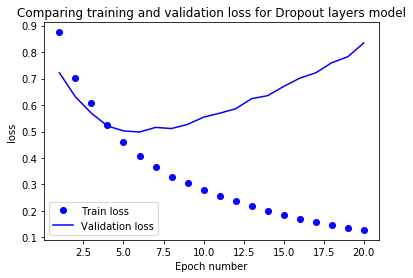
The model with dropout layers starts overfitting later than the baseline model. The loss also increases slower than the baseline model.
compare_models_by_metric(base_model, drop_model, base_history, drop_history, 'val_loss')
The model with the dropout layers starts overfitting later. Compared to the baseline model the loss also remains much lower.
Training on the full train data and evaluation on test data
At first sight, the reduced model seems to be the best model for generalization. But let’s check that on the test set.
base_results = test_model(base_model, X_train_oh, y_train_oh, X_test_oh, y_test_oh, base_min)
reduced_results = test_model(reduced_model, X_train_oh, y_train_oh, X_test_oh, y_test_oh, reduced_min)
reg_results = test_model(reg_model, X_train_oh, y_train_oh, X_test_oh, y_test_oh, reg_min)
drop_results = test_model(drop_model, X_train_oh, y_train_oh, X_test_oh, y_test_oh, drop_min)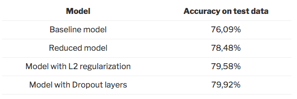
Conclusion
As shown above, all three options help to reduce overfitting. We manage to increase the accuracy on the test data substantially. Among these three options, the model with the dropout layers performs the best on the test data.
You can find the notebook on GitHub. Have fun with it!