
One of machine learning's most popular applications is in solving classification problems.
Classification problems are situations where you have a data set, and you want to classify observations from that data set into a specific category.
A famous example is a spam filter for email providers. Gmail uses supervised machine learning techniques to automatically place emails in your spam folder based on their content, subject line, and other features.
Two machine learning models perform much of the heavy lifting when it comes to classification problems:
- K-nearest neighbors
- K-means clustering
This tutorial will teach you how to code K-nearest neighbors and K-means clustering algorithms in Python.
K-Nearest Neighbors Models
The K-nearest neighbors algorithm is one of the world’s most popular machine learning models for solving classification problems.
A common exercise for students exploring machine learning is to apply the K nearest neighbors algorithm to a data set where the categories are not known. A real-life example of this would be if you needed to make predictions using machine learning on a data set of classified government information.
In this tutorial, you will learn to write your first K nearest neighbors machine learning algorithm in Python. We will be working with an anonymous data set similar to the situation described above.
The Data Set You Will Need in This Tutorial
The first thing you need to do is download the data set we will be using in this tutorial. I have uploaded the file to my website. You can access it by clicking here.
Now that you have downloaded the data set, you will want to move the file to the directory that you’ll be working in. After that, open a Jupyter Notebook and we can get started writing Python code!
The Libraries You Will Need in This Tutorial
To write a K nearest neighbors algorithm, we will take advantage of many open-source Python libraries including NumPy, pandas, and scikit-learn.
Begin your Python script by writing the following import statements:
import numpy as np

import pandas as pd

import matplotlib.pyplot as plt

import seaborn as sns

%matplotlib inline
Importing the Data Set Into Our Python Script
Our next step is to import the classified_data.csv file into our Python script. The pandas library makes it easy to import data into a pandas DataFrame.
Since the data set is stored in a csv file, we will be using the read_csv method to do this:
raw_data = pd.read_csv('classified_data.csv')
Printing this DataFrame inside of your Jupyter Notebook will give you a sense of what the data looks like:
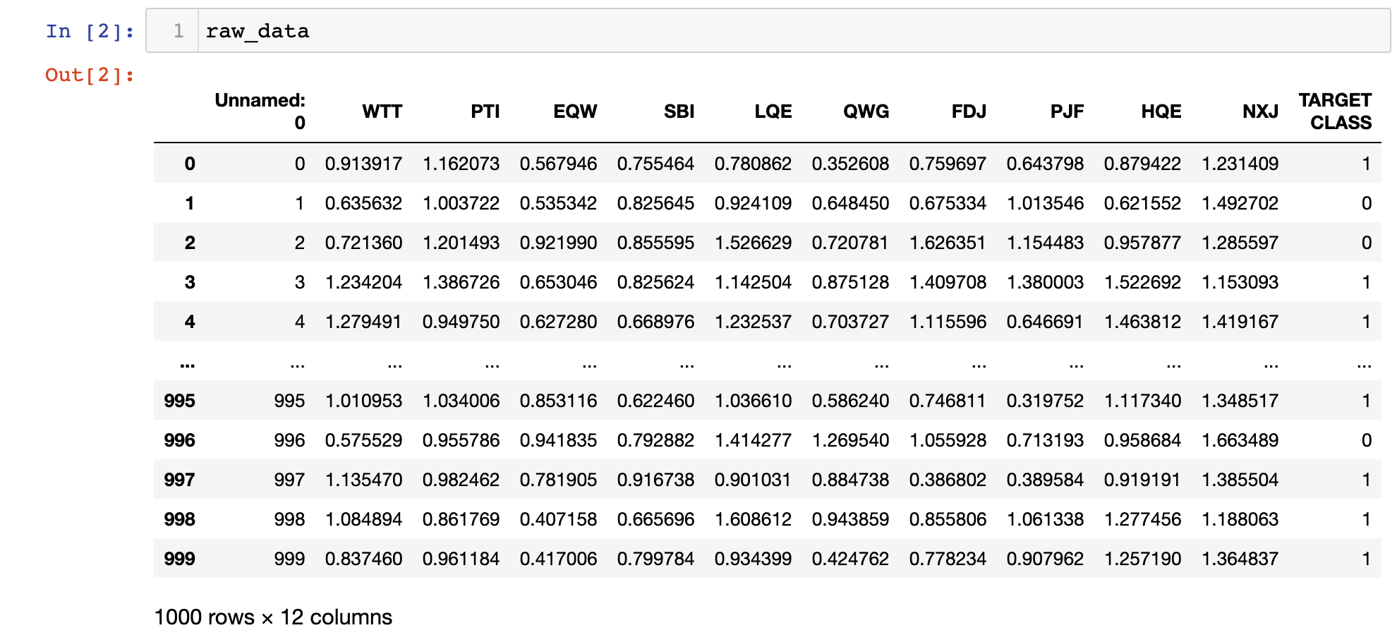
You will notice that the DataFrame starts with an unnamed column whose values are equal to the DataFrame’s index. We can fix this by making a slight adjustment to the command that imported our data set into the Python script:
raw_data = pd.read_csv('classified_data.csv', index_col = 0)
Next, let’s take a look at the actual features that are contained in this data set. You can print a list of the data set’s column names with the following statement:
print(raw_data.columns)
This returns:
Index(['WTT', 'PTI', 'EQW', 'SBI', 'LQE', 'QWG', 'FDJ', 'PJF', 'HQE', 'NXJ',

       'TARGET CLASS'],

      dtype='object')
Since this is a classified data set, we have no idea what any of these columns means. For now, it is sufficient to recognize that every column is numerical in nature and thus well-suited for modelling with machine learning techniques.
Standardizing the Data Set
Since the K nearest neighbors algorithm makes predictions about a data point by using the observations that are closest to it, the scale of the features within a data set matters a lot.
Because of this, machine learning practitioners typically standardize the data set, which means adjusting every x value so that they are roughly on the same scale.
Fortunately, scikit-learn includes some excellent functionality to do this with very little headache.
To start, we will need to import the StandardScaler class from scikit-learn. Add the following command to your Python script to do this:
from sklearn.preprocessing import StandardScaler
This function behaves a lot like the LinearRegression and LogisticRegression classes that we used earlier in this course. We will want to create an instance of this class and then fit the instance of that class on our data set.
First, let’s create an instance of the StandardScaler class named scaler with the following statement:
scaler = StandardScaler()
We can now train this instance on our data set using the fit method:
scaler.fit(raw_data.drop('TARGET CLASS', axis=1))
Now we can use the transform method to standardize all of the features in the data set so they are roughly the same scale. We’ll assign these scaled features to the variable named scaled_features:
scaled_features = scaler.transform(raw_data.drop('TARGET CLASS', axis=1))
This actually creates a NumPy array of all the features in the data set, and we want it to be a pandas DataFrame instead.
Fortunately, this is an easy fix. We’ll simply wrap the scaled_features variable in a pd.DataFrame method and assign this DataFrame to a new variable called scaled_data with an appropriate argument to specify the column names:
scaled_data = pd.DataFrame(scaled_features, columns = raw_data.drop('TARGET CLASS', axis=1).columns)
Now that we have imported our data set and standardized its features, we are ready to split the data set into training data and test data.
Splitting the Data Set Into Training Data and Test Data
We will use the train_test_split function from scikit-learn combined with list unpacking to create training data and test data from our classified data set.
First, you’ll need to import train_test_split from the model_validation module of scikit-learn with the following statement:
from sklearn.model_selection import train_test_split
Next, we will need to specify the x and y values that will be passed into this train_test_split function.
The x values will be the scaled_data DataFrame that we created previously. The y values will be the TARGET CLASS column of our original raw_data DataFrame.
You can create these variables with the following statements:
x = scaled_data

y = raw_data['TARGET CLASS']
Next, you’ll need to run the train_test_split function using these two arguments and a reasonable test_size. We will use a test_size of 30%, which gives the following parameters for the function:
x_training_data, x_test_data, y_training_data, y_test_data = train_test_split(x, y, test_size = 0.3)
Now that our data set has been split into training data and test data, we’re ready to start training our model!
Training a K Nearest Neighbors Model
Let’s start by importing the KNeighborsClassifier from scikit-learn:
from sklearn.neighbors import KNeighborsClassifier
Next, let’s create an instance of the KNeighborsClassifier class and assign it to a variable named model
This class requires a parameter named n_neighbors, which is equal to the K value of the K nearest neighbors algorithm that you’re building. To start, let’s specify n_neighbors = 1:
model = KNeighborsClassifier(n_neighbors = 1)
Now we can train our K nearest neighbors model using the fit method and our x_training_data and y_training_data variables:
model.fit(x_training_data, y_training_data)
Now let’s make some predictions with our newly-trained K nearest neighbors algorithm!
Making Predictions With Our K Nearest Neighbors Algorithm
We can make predictions with our K nearest neighbors algorithm in the same way that we did with our linear regression and logistic regression models earlier in this course: by using the predict method and passing in our x_test_data variable.
More specifically, here’s how you can make predictions and assign them to a variable called predictions:
predictions = model.predict(x_test_data)
Let’s explore how accurate our predictions are in the next section of this tutorial.
Measuring the Accuracy of Our Model
We saw in our logistic regression tutorial that scikit-learn comes with built-in functions that make it easy to measure the performance of machine learning classification models.
Let’s import two of these functions (classification_report and confuson_matrix) into our report now:
from sklearn.metrics import classification_report

from sklearn.metrics import confusion_matrix
Let’s work through each of these one-by-one, starting with the classfication_report. You can generate the report with the following statement:
print(classification_report(y_test_data, predictions))
This generates:
             precision    recall  f1-score   support

           0       0.94      0.85      0.89       150

           1       0.86      0.95      0.90       150

    accuracy                           0.90       300

   macro avg       0.90      0.90      0.90       300

weighted avg       0.90      0.90      0.90       300
Similarly, you can generate a confusion matrix with the following statement:
print(confusion_matrix(y_test_data, predictions))
This generates:
[[141  12]

 [ 18 129]]
Looking at these performance metrics, it looks like our model is already fairly performant. It can still be improved.
In the next section, we will see how we can improve the performance of our K nearest neighbors model by choosing a better value for K.
Choosing An Optimal K Value Using the Elbow Method
In this section, we will use the elbow method to choose an optimal value of K for our K nearest neighbors algorithm.
The elbow method involves iterating through different K values and selecting the value with the lowest error rate when applied to our test data.
To start, let’s create an empty list called error_rates. We will loop through different K values and append their error rates to this list.
error_rates = []
Next, we need to make a Python loop that iterates through the different values of K we’d like to test and executes the following functionality with each iteration:
- Creates a new instance of the
KNeighborsClassifierclass fromscikit-learn - Trains the new model using our training data
- Makes predictions on our test data
- Calculates the mean difference for every incorrect prediction (the lower this is, the more accurate our model is)
Here is the code to do this for K values between 1 and 100:
for i in np.arange(1, 101):

    new_model = KNeighborsClassifier(n_neighbors = i)

    new_model.fit(x_training_data, y_training_data)

    new_predictions = new_model.predict(x_test_data)

    error_rates.append(np.mean(new_predictions != y_test_data))
Let’s visualize how our error rate changes with different K values using a quick matplotlib visualization:
plt.plot(error_rates)
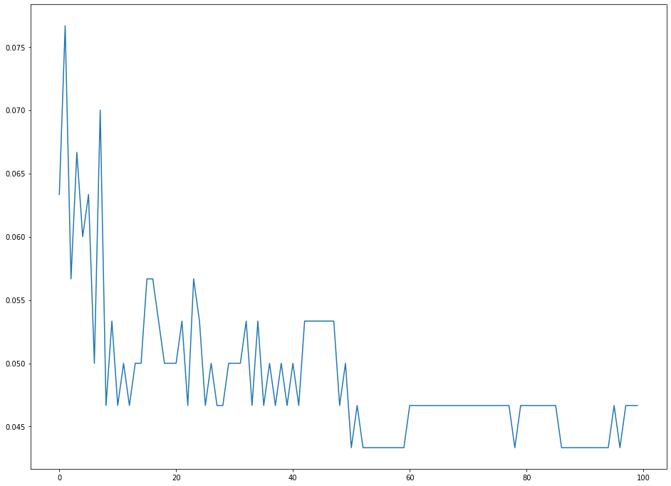
As you can see, our error rates tend to be minimized with a K value of approximately 50. This means that 50 is a suitable choice for K that balances both simplicity and predictive power.
The Full Code For This Tutorial
You can view the full code for this tutorial in this GitHub repository. It is also pasted below for your reference:
#Common imports

import numpy as np

import pandas as pd

import matplotlib.pyplot as plt

import seaborn as sns

%matplotlib inline

#Import the data set

raw_data = pd.read_csv('classified_data.csv', index_col = 0)

#Import standardization functions from scikit-learn

from sklearn.preprocessing import StandardScaler

#Standardize the data set

scaler = StandardScaler()

scaler.fit(raw_data.drop('TARGET CLASS', axis=1))

scaled_features = scaler.transform(raw_data.drop('TARGET CLASS', axis=1))

scaled_data = pd.DataFrame(scaled_features, columns = raw_data.drop('TARGET CLASS', axis=1).columns)

#Split the data set into training data and test data

from sklearn.model_selection import train_test_split

x = scaled_data

y = raw_data['TARGET CLASS']

x_training_data, x_test_data, y_training_data, y_test_data = train_test_split(x, y, test_size = 0.3)

#Train the model and make predictions

from sklearn.neighbors import KNeighborsClassifier

model = KNeighborsClassifier(n_neighbors = 1)

model.fit(x_training_data, y_training_data)

predictions = model.predict(x_test_data)

#Performance measurement

from sklearn.metrics import classification_report

from sklearn.metrics import confusion_matrix

print(classification_report(y_test_data, predictions))

print(confusion_matrix(y_test_data, predictions))

#Selecting an optimal K value

error_rates = []

for i in np.arange(1, 101):

    new_model = KNeighborsClassifier(n_neighbors = i)

    new_model.fit(x_training_data, y_training_data)

    new_predictions = new_model.predict(x_test_data)

    error_rates.append(np.mean(new_predictions != y_test_data))

plt.figure(figsize=(16,12))

plt.plot(error_rates)
K-Means Clustering Models
The K-means clustering algorithm is typically the first unsupervised machine learning model that students will learn.
It allows machine learning practitioners to create groups of data points within a data set with similar quantitative characteristics. It is useful for solving problems like creating customer segments or identifying localities in a city with high crime rates.
In this section, you will learn how to build your first K means clustering algorithm in Python.
The Data Set We Will Use In This Tutorial
In this tutorial, we will be using a data set of data generated using scikit-learn.
Let’s import scikit-learn’s make_blobs function to create this artificial data. Open up a Jupyter Notebook and start your Python script with the following statement:
from sklearn.datasets import make_blobs
Now let’s use the make_blobs function to create some artificial data!
More specifically, here is how you could create a data set with 200 samples that has 2 features and 4 cluster centers. The standard deviation within each cluster will be set to 1.8.
raw_data = make_blobs(n_samples = 200, n_features = 2, centers = 4, cluster_std = 1.8)
If you print this raw_data object, you’ll notice that it is actually a Python tuple. The first element of this tuple is a NumPy array with 200 observations. Each observation contains 2 features (just like we specified with our make_blobs function!).
Now that our data has been created, we can move on to importing other important open-source libraries into our Python script.
The Imports We Will Use In This Tutorial
This tutorial will make use of a number of popular open-source Python libraries, including pandas, NumPy, and matplotlib. Let’s continue our Python script by adding the following imports:
import pandas as pd

import numpy as np

import seaborn

import matplotlib.pyplot as plt

%matplotlib inline
The first group of imports in this code block is for manipulating large data sets. The second group of imports is for creating data visualizations.
Let’s move on to visualizing our data set next.
Visualizing Our Data Set
In our make_blobs function, we specified for our data set to have 4 cluster centers. The best way to verify that this has been handled correctly is by creating some quick data visualizations.
To start, let’s use the following command to plot all of the rows in the first column of our data set against all of the rows in the second column of our data set:
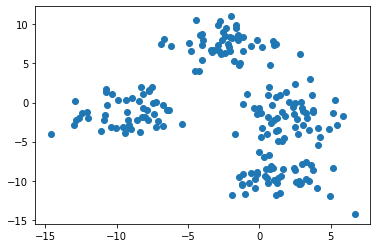
Note: your data set will appear differently than mine since this is randomly-generated data.
This image seems to indicate that our data set has only three clusters. This is because two of the clusters are very close to each other.
To fix this, we need to reference the second element of our raw_data tuple, which is a NumPy array that contains the cluster to which each observation belongs.
If we color our data set using each observation’s cluster, the unique clusters will quickly become clear. Here is the code to do this:
plt.scatter(raw_data[0][:,0], raw_data[0][:,1], c=raw_data[1])
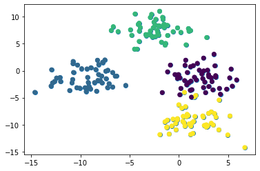
We can now see that our data set has four unique clusters. Let’s move on to building our K means cluster model in Python!
Building and Training Our K Means Clustering Model
The first step to building our K means clustering algorithm is importing it from scikit-learn. To do this, add the following command to your Python script:
from sklearn.cluster import KMeans
Next, lets create an instance of this KMeans class with a parameter of n_clusters=4 and assign it to the variable model:
model = KMeans(n_clusters=4)
Now let’s train our model by invoking the fit method on it and passing in the first element of our raw_data tuple:
model.fit(raw_data[0])
In the next section, we’ll explore how to make predictions with this K means clustering model.
Before moving on, I wanted to point out one difference that you may have noticed between the process for building this K means clustering algorithm (which is an unsupervised machine learning algorithm) and the supervised machine learning algorithms we’ve worked with so far in this course.
Namely, we did not have to split the data set into training data and test data. This is an important difference - and in fact, you never need to make the train/test split on a data set when building unsupervised machine learning models!
Making Predictions With Our K Means Clustering Model
Machine learning practitioners generally use K means clustering algorithms to make two types of predictions:
- Which cluster each data point belongs to
- Where the center of each cluster is
It is easy to generate these predictions now that our model has been trained.
First, let’s predict which cluster each data point belongs to. To do this, access the labels_ attribute from our model object using the dot operator, like this:
model.labels_
This generates a NumPy array with predictions for each data point that looks like this:
array([3, 2, 7, 0, 5, 1, 7, 7, 6, 1, 2, 4, 6, 7, 6, 4, 4, 3, 3, 6, 0, 0,

       6, 4, 5, 6, 0, 2, 6, 5, 4, 3, 4, 2, 6, 6, 6, 5, 6, 2, 1, 1, 3, 4,

       3, 5, 7, 1, 7, 5, 3, 6, 0, 3, 5, 5, 7, 1, 3, 1, 5, 7, 7, 0, 5, 7,

       3, 4, 0, 5, 6, 5, 1, 4, 6, 4, 5, 6, 7, 2, 2, 0, 4, 1, 1, 1, 6, 3,

       3, 7, 3, 6, 7, 7, 0, 3, 4, 3, 4, 0, 3, 5, 0, 3, 6, 4, 3, 3, 4, 6,

       1, 3, 0, 5, 4, 2, 7, 0, 2, 6, 4, 2, 1, 4, 7, 0, 3, 2, 6, 7, 5, 7,

       5, 4, 1, 7, 2, 4, 7, 7, 4, 6, 6, 3, 7, 6, 4, 5, 5, 5, 7, 0, 1, 1,

       0, 0, 2, 5, 0, 3, 2, 5, 1, 5, 6, 5, 1, 3, 5, 1, 2, 0, 4, 5, 6, 3,

       4, 4, 5, 6, 4, 4, 2, 1, 7, 4, 6, 6, 0, 6, 3, 5, 0, 5, 2, 4, 6, 0,

       1, 0], dtype=int32)
To see where the center of each cluster lies, access the cluster_centers_ attribute using the dot operator like this:
model.cluster_centers_
This generates a two-dimensional NumPy array that contains the coordinates of each clusters center. It will look like this:
array([[ -8.06473328,  -0.42044783],

       [  0.15944397,  -9.4873621 ],

       [  1.49194628,   0.21216413],

       [-10.97238157,  -2.49017206],

       [  3.54673215,  -9.7433692 ],

       [ -3.41262049,   7.80784834],

       [  2.53980034,  -2.96376999],

       [ -0.4195847 ,   6.92561289]])
We’ll assess the accuracy of these predictions in the next section.
Visualizing the Accuracy of Our Model
The last thing we’ll do in this tutorial is visualize the accuracy of our model. You can use the following code to do this:
f, (ax1, ax2) = plt.subplots(1, 2, sharey=True,figsize=(10,6))

ax1.set_title('Our Model')

ax1.scatter(raw_data[0][:,0], raw_data[0][:,1],c=model.labels_)

ax2.set_title('Original Data')

ax2.scatter(raw_data[0][:,0], raw_data[0][:,1],c=raw_data[1])
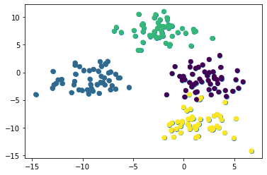
This generates two different plots side-by-side where one plot shows the clusters according to the real data set and the other plot shows the clusters according to our model. Here is what the output looks like:
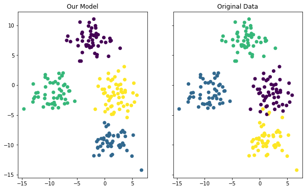
Although the coloring between the two plots is different, you can see that our model did a fairly good job of predicting the clusters within our data set. You can also see that the model was not perfect - if you look at the data points along a cluster’s edge, you can see that it occasionally misclassified an observation from our data set.
There’s one last thing that needs to be mentioned about measuring our model’s prediction. In this example ,we knew which cluster each observation belonged to because we actually generated this data set ourselves.
This is highly unusual. K means clustering is more often applied when the clusters aren’t known in advance. Instead, machine learning practitioners use K means clustering to find patterns that they don’t already know within a data set.
The Full Code For This Tutorial
You can view the full code for this tutorial in this GitHub repository. It is also pasted below for your reference:
#Create artificial data set

from sklearn.datasets import make_blobs

raw_data = make_blobs(n_samples = 200, n_features = 2, centers = 4, cluster_std = 1.8)

#Data imports

import pandas as pd

import numpy as np

#Visualization imports

import seaborn

import matplotlib.pyplot as plt

%matplotlib inline

#Visualize the data

plt.scatter(raw_data[0][:,0], raw_data[0][:,1])

plt.scatter(raw_data[0][:,0], raw_data[0][:,1], c=raw_data[1])

#Build and train the model

from sklearn.cluster import KMeans

model = KMeans(n_clusters=4)

model.fit(raw_data[0])

#See the predictions

model.labels_

model.cluster_centers_

#PLot the predictions against the original data set

f, (ax1, ax2) = plt.subplots(1, 2, sharey=True,figsize=(10,6))

ax1.set_title('Our Model')

ax1.scatter(raw_data[0][:,0], raw_data[0][:,1],c=model.labels_)

ax2.set_title('Original Data')

ax2.scatter(raw_data[0][:,0], raw_data[0][:,1],c=raw_data[1])
Final Thoughts
This tutorial taught you how to how to build K-nearest neighbors and K-means clustering machine learning models in Python.
If you're interested in learning more about machine learning, my book Pragmatic Machine Learning will teach you practical machine learning techniques by building 9 real projects. The book launches August 3rd. You can preorder it for 50% off using the link below:

Here is a brief summary of what you learned about K-nearest neighbors models in Python:
- How classified data is a common tool used to teach students how to solve their first K nearest neighbor problems
- Why it’s important to standardize your data set when building K nearest neighbor models
- How to split your data set into training data and test data using the
train_test_splitfunction - How to train your first K nearest neighbors model and make predictions with it
- How to measure the performance of a K nearest neighbors model
- How to use the elbow method to select an optimal value of K in a K nearest neighbors model
Similarly, here is a brief summary of what you learned about K-means clustering models in Python:
- How to create artificial data in
scikit-learnusing themake_blobsfunction - How to build and train a K means clustering model
- That unsupervised machine learning techniques do not require you to split your data into training data and test data
- How to build and train a K means clustering model using
scikit-learn - How to visualizes the performance of a K means clustering algorithm when you know the clusters in advance