
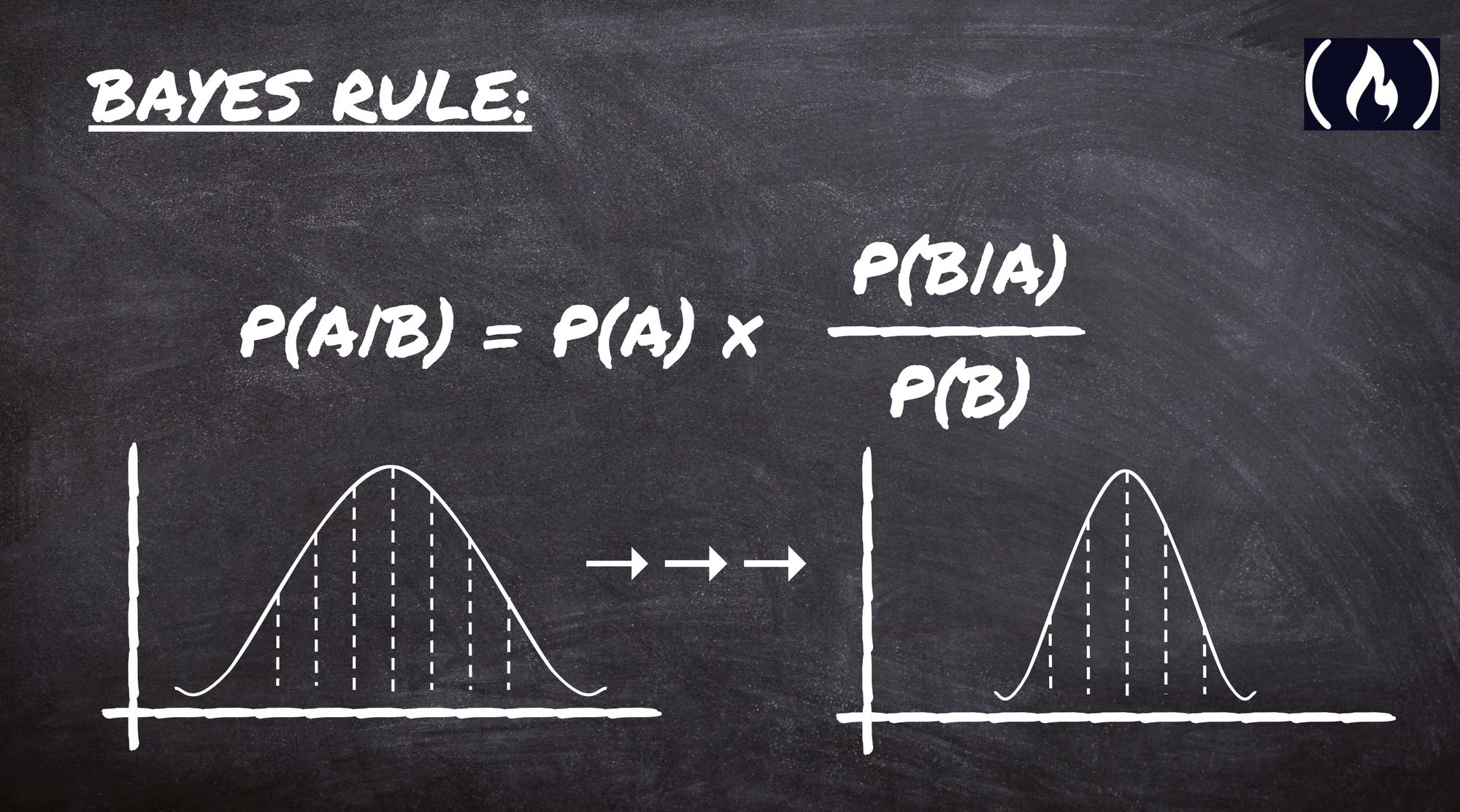
Bayes' Rule is the most important rule in data science. It is the mathematical rule that describes how to update a belief, given some evidence. In other words – it describes the act of learning.
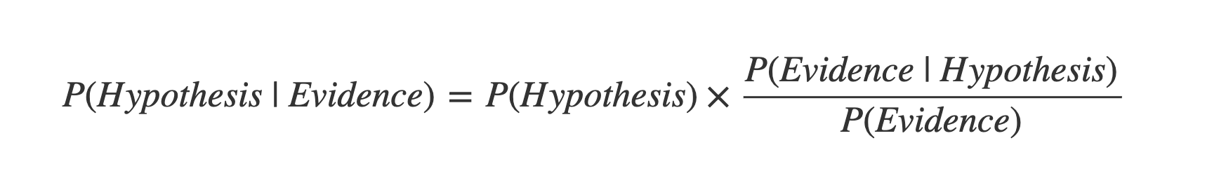
The equation itself is not too complex:
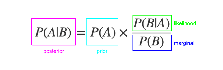
There are four parts:
- Posterior probability (updated probability after the evidence is considered)
- Prior probability (the probability before the evidence is considered)
- Likelihood (probability of the evidence, given the belief is true)
- Marginal probability (probability of the evidence, under any circumstance)
Bayes' Rule can answer a variety of probability questions, which help us (and machines) understand the complex world we live in.
It is named after Thomas Bayes, an 18th century English theologian and mathematician. Bayes originally wrote about the concept, but it did not receive much attention during his lifetime.
French mathematician Pierre-Simon Laplace independently published the rule in his 1814 work Essai philosophique sur les probabilités.
Today, Bayes' Rule has numerous applications, from statistical analysis to machine learning.
This article will explain Bayes' Rule in plain language.
Conditional probability
The first concept to understand is conditional probability.
You may already be familiar with probability in general. It lets you reason about uncertain events with the precision and rigour of mathematics.
Conditional probability is the bridge that lets you talk about how multiple uncertain events are related. It lets you talk about how the probability of an event can vary under different conditions.
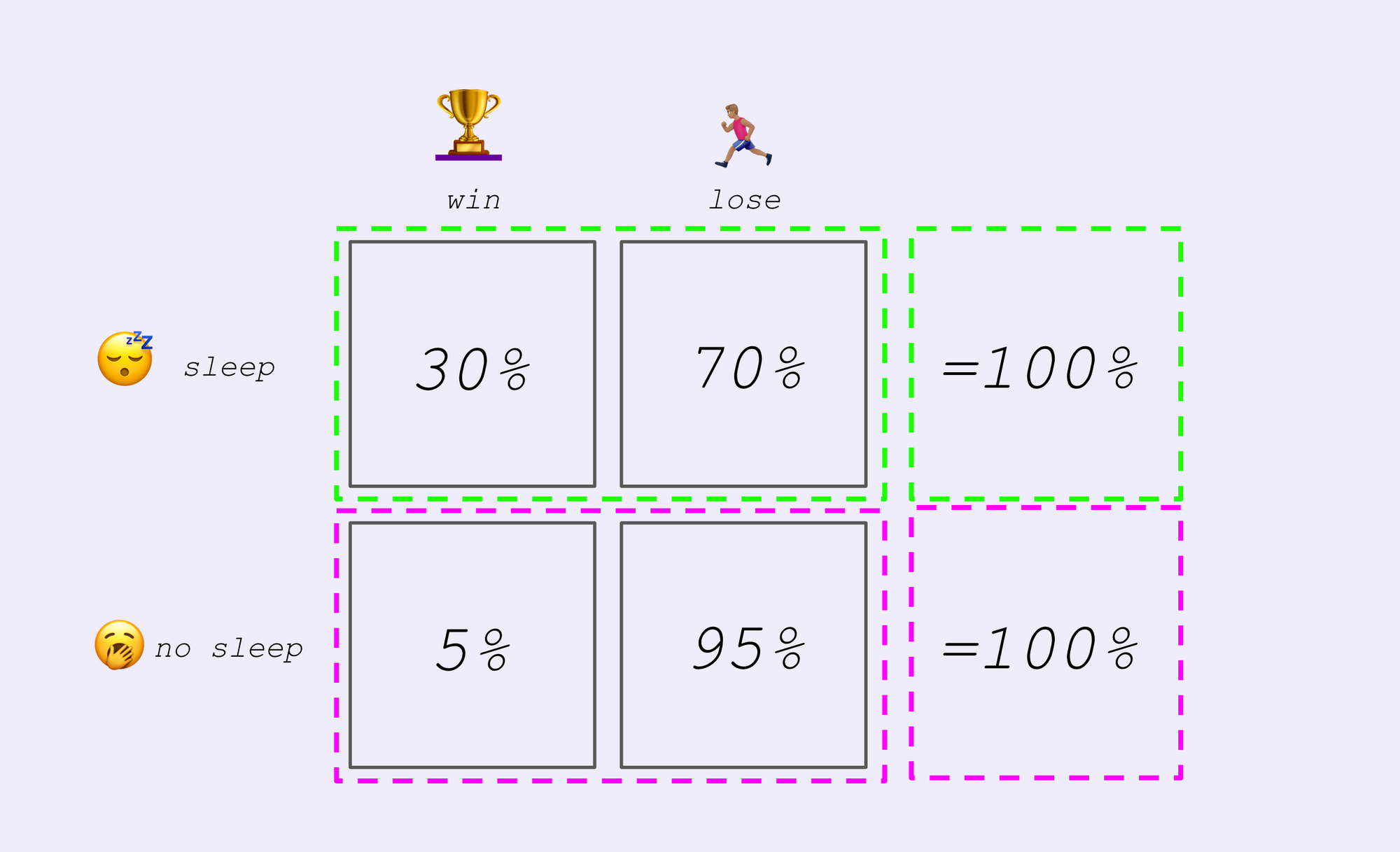
For example, consider the probability of winning a race, given the condition you didn't sleep the night before. You might expect this probability to be lower than the probability you'd win if you'd had a full night's sleep.
Or, consider the probability that a suspect committed a crime, given that their fingerprints are found at the scene. You'd expect the probability they are guilty to be greater, compared with had their fingerprints not been found.
The notation for conditional probability is usually:
Which is read as "the probability of event A occurring, given event B occurs".
An important thing to remember is that conditional probabilities are not the same as their inverses.
That is, the "probability of event A given event B" is not the same thing as the "probability of event B, given event A".
To remember this, take the following example:
The probability of clouds, given it is raining (100%) is not the same as the probability it is raining, given there are clouds.
(Insert joke about British weather).
Bayes' Rule in detail
Bayes' Rule tells you how to calculate a conditional probability with information you already have.
It is helpful to think in terms of two events – a hypothesis (which can be true or false) and evidence (which can be present or absent).
However, it can be applied to any type of events, with any number of discrete or continuous outcomes.
Bayes' Rule lets you calculate the posterior (or "updated") probability. This is a conditional probability. It is the probability of the hypothesis being true, if the evidence is present.
Think of the prior (or "previous") probability as your belief in the hypothesis before seeing the new evidence. If you had a strong belief in the hypothesis already, the prior probability will be large.
The prior is multiplied by a fraction. Think of this as the "strength" of the evidence. The posterior probability is greater when the top part (numerator) is big, and the bottom part (denominator) is small.
The numerator is the likelihood. This is another conditional probability. It is the probability of the evidence being present, given the hypothesis is true.
This is not the same as the posterior!
Remember, the "probability of the evidence being present given the hypothesis is true" is not the same as the "probability of the hypothesis being true given the evidence is present".
Now look at the denominator. This is the marginal probability of the evidence. That is, it is the probability of the evidence being present, whether the hypothesis is true or false. The smaller the denominator, the more "convincing" the evidence.
Worked example of Bayes' Rule
Here's a simple worked example.
Your neighbour is watching their favourite football (or soccer) team. You hear them cheering, and want to estimate the probability their team has scored.
Step 1 – write down the posterior probability of a goal, given cheering
Step 2 – estimate the prior probability of a goal as 2%
Step 3 – estimate the likelihood probability of cheering, given there's a goal as 90% (perhaps your neighbour won't celebrate if their team is losing badly)
Step 4 – estimate the marginal probability of cheering – this could be because:
- a goal has been scored (2% of the time, times 90% probability)
- or any other reason, such as the other team missing a penalty or having a player sent off (98% of the time, times perhaps 1% probability)
Now, piece everything together:

Use cases for Bayes' Rule and next steps
Bayes' Rule has use cases in many areas:
- Understanding probability problems (including those in medical research)
- Statistical modelling and inference
- Machine learning algorithms (such as Naive Bayes, Expectation Maximisation)
- Quantitative modelling and forecasting
Next, you'll discover how Bayes' Rule can be used to quantify uncertainty and model real world problems. Then, how to reason about "probabilities of probabilities".
The final step will cover how various computational tricks let you make use of Bayes' Rule to solve non-trivial problems.