
By Déborah Mesquita
A primer on Inferential statistics and how to extract information from text using spaCy

In Data Science we usually talk a lot about Exploratory Data Analysis (Descriptive Statistics), but there is another “statistical world” that can also be very useful: the world of Inferential Statistics.
Inferential statistical analysis infers properties of a population, for example by testing hypotheses and deriving estimates. Descriptive statistics is solely concerned with properties of the observed data, and it does not rest on the assumption that the data come from a larger population. — Statistical Inference
In this article we’ll use the gitter-history dataset from freeCodeCamp open data to answer this question: is there a different mention pattern in the chat-rooms from different cities?
We’ll learn about inferential statistics and also learn how to extract information from text using the Matcher class from spaCy. First let’s extract the data, then we’ll get our hands dirty with statistics (hey, it’s fun! you’ll see).
Extracting information with spacy.Matcher
The way we use the Matcher is very similar to the way we use regular expressions (in fact we can use regex to create patterns). Each rule can have many patterns, and a pattern consists of a list of dicts, where each dict describes a token.
// this pattern matches all tokens == 'hello' (lowercase){'LOWER': 'hello'}
Let’s create some examples of things we can extract from the messages.
Greetings
Here we have 4 patterns for the same rule ("GREETINGS"):
matcher = Matcher(nlp.vocab)
self.matcher.add("GREETINGS", None, [{"LOWER": "good"}, {"LOWER": "morning"}], [{"LOWER": "good"}, {"LOWER": "evening"}], [{"LOWER": "good"}, {"LOWER": "afternoon"}], [{"LOWER": "good"}, {"LOWER": "night"}])
matches = matcher(text)
Messages with punctuation
We can use all the available token attributes as patterns. Let’s see if a message has a punctuation token.
matcher = Matcher(nlp.vocab)
self.matcher.add("PUNCT", None, [{"IS_PUNCT": True}])
matches = matcher(text)
What are people feeling?
Here things get a little more interesting. We’ll match the lemma of the verb be to detect all the conjugations of the verb. The matcher also lets you use quantifiers, specified as the 'OP' key. We’ll match all the adverb tokens after the verb be (with 'OP': '*' we can match any and all of them).
After that there is a lot of possibility for the two following words, so we’ll use the wildcard token {} to match them.
matcher = Matcher(nlp.vocab)
self.matcher.add("FEELING", None, [ {"LOWER": "i"}, {"LEMMA":"be"}, {"POS": "ADV", "OP": "*"}, {"POS": "ADJ"} ])
matches = matcher(text)
Mentions
There is not a token attribute to @some_token, so let’s create one.
mention_flag = lambda text: bool(re.compile(r'\@(\w+)').match(text))
IS_MENTION = nlp.vocab.add_flag(mention_flag)
self.matcher.add("MENTION", None, [{IS_MENTION: True}])
matches = matcher(text)
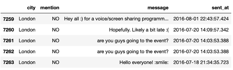
I built a dataset with mentions for the rest of the article.
[menssage, mention, sent_at, city]
You can find all the code here.
A primer on Inferential statistics
Statistical inference is the process of using data analysis to deduce properties of an underlying probability distribution (Statistical inference).
We have samples and we want to compare them. With Test Statistic we can measure the probability of they coming from the same distribution or not. Applying this to our scenario, if the probability of the mentions coming from the same distribution is below a threshold (defined by us) then we’ll be able to infer that people from different cities have different mention patterns.
Let’s define some concepts to clarify things (all the definitions are taken from Wikipedia):
- Frequency distribution: a list, table or graph that displays the frequency of various outcomes in a sample
- Null hypothesis: a general statement or default position that there is no relationship between two measured phenomena, or no association among groups
- p-value: the probability, when the null hypothesis is true, of obtaining a result equal to or more extreme than what was actually observed. The smaller the p-value, the higher the significance because it tells the investigator that the hypothesis under consideration may not adequately explain the observation
- Statistical significance: something is statistically significant if it allows us to reject the null hypothesis
One thing to keep in mind while dealing with statistical hypothesis tests is that it goes like this:
- We assume something is true
- Then we try to prove that it’s impossible that it can be true
- Then when we see that indeed, this probably can’t be true for the results we got, we reject the claim
“Null hypothesis testing is a reductio ad absurdum argument adapted to statistics. In essence, a claim is assumed valid if its counter-claim is improbable”. — P-value
In our case we are dealing with categorical variables (a variable that can take on one of a limited, and usually fixed number of possible values). Because of that, we’ll use the Chi-squared distribution.
In probability theory and statistics, the chi-squared distribution (also chi-square or _χ_2-distribution) with k degrees of freedom is the distribution of a sum of the squares of k independent standard normal random variables. It’s one of the most widely used probability distributions in inferential statistics, notably in hypothesis testing or in construction of confidence intervals. — Chi-squared distribution
“Statisticians have identified several common distributions, known as probability distributions. From these distributions it is possible to calculate the probability of getting particular scores based on the frequencies with which a particular score occurs in a distribution with these common shapes.” — Discovering Statistics Using R
Understanding the chi-square test for homogeneity
We want to know if the mention distribution is the same for each city. First we assume that they indeed come from the same population, then we get all the messages from each city and sum them up. This distribution (all the messages together) should be the same for each city if we assume they come from the same population.
We cannot prove that the distributions are different using statistics, but we can reject that they are the same.
“The reason that we need the null hypothesis is because we cannot prove the experimental hypothesis using statistics, but we can reject the null hypothesis. If our data give us confidence to reject the null hypothesis then this provides support for our experimental hypothesis. However, be aware that even if we can reject the null hypothesis, this doesn’t prove the experimental hypothesis — it merely supports it.” — Discovering Statistics Using R
This is very important. We are not proving that the experimental (or alternative) hypothesis is true. We are saying that at a given significance level it’s likely that it’s true.
“So, rather than talking about accepting or rejecting a hypothesis (which some textbooks tell you to do) we should be talking about ‘the chances of obtaining the data we’ve collected assuming that the null hypothesis is true’.” — Discovering Statistics Using R
In essence, when we collect data to test theories we can only talk in terms of the probability of obtaining a particular set of data (Field, Andy). And to judge that we use the p-values.
- High p-values: your data are likely with a true null
- Low p-values: your data are unlikely with a true null, (How to Correctly Interpret P Values)
We’ll set our significance level to 5% (p-value threshold of 0.05).
Ok, now back to the test.
The data
We’ll use the dataset of all chat activity in freeCodeCamp’s Gitter chatrooms. This dataset can be found here.
Our sample has all messages from the San Francisco, Toronto, Boston, Belgrade, London and Sao Paulo sent between 2015–08–16 and 2016–08–16 (one year of messages).
Conditions for conducting the chi-square test for homogeneity
To use the chi-square test we need to meet some conditions:
- For each population, the sampling method is simple random sampling
- All of the expected counts are 5 or greater
We’ll assume the first condition is met (1 year of data from each city). Let’s find out if the second condition is met.
Exploring the data
Since we are sipping at the waters of statistics let’s use R instead of Python.
I created a JSON file and we’ll load it into a dataframe using the jsonlite library. To see the contents we’ll use the tally function.
> library(jsonlite)
> df <- fromJSON("experiment_sample_data.json")
> library(mosaic)
> mentiontable <- tally(~city+mention, data=df, margins=T)> mentiontable mentioncity NO YES Belgrade 184 45 Boston 383 121 London 278 98 SanFrancisco 156 51 SaoPaulo 153 132 Toronto 379 81
Now is the time to introduce the contingency tables.
- Contingency tables: in statistics, a contingency table (also known as a cross tabulation or crosstab) is a type of table in a matrix format that displays the (multivariate) frequency distribution of the variables.
With chisq.test we can perform chi-squared contingency table tests and goodness-of-fit tests. Let’s calculate the expected counts for this sample.
Expected outcome = (sum of data in that row)×(sum of data in that column) / total data.
So the expected number of messages with mentions (mention=YES) for the city of Sao Paulo is:
285407/1557 = *74,49903
The expected value of chisq.test gives the expected counts under the null hypothesis for all the cities:
> chisq.test(mentiontable)$expected mentioncity NO YES Belgrade 170.3333 58.66667 Boston 374.8821 129.11790 London 279.6739 96.32606 SanFrancisco 153.9694 53.03057 SaoPaulo 211.9869 73.01310 Toronto 342.1543 117.84571
The expected counts are all greater than 5, so we can perform the test.
Performing the chi-square test
We’ll assume the distributions are the same, so the total column is the best estimate of what this distribution should be:
> tally(~mention, data=df)mention NO YES 1150 407
The chi-squared test is used to determine whether there is a significant difference between the expected frequencies and the observed frequencies.
For each cell, the expected frequency is subtracted from the observed frequency, the difference is squared, and the total is divided by the expected frequency. The values are then summed across all cells. This sum is the chi-square test statistic — The chi-square test
With the value from the chi-square test and with the value for the degrees of freedom (number_if_rows -1 × number_of_columns -1) we can calculate the probability of getting the results by chance or not.
> chisq.test(mentiontable) Pearson's Chi-squared test
data: mentiontableX-squared = 84.667, df = 5, p-value < 2.2e-16
The p-value is lower than the alpha value (0.05), so we will reject the null hypothesis. This means that with these results for each city, it is unlikely that all the cities have the same distribution of mentions.
We can also examine the source of differences of the test.
Examining residuals for the source of differences
We have the expected values for each city, so it’s possible to see the residuals: (observed - expected) / sqrt(expected)
The standardized residual, provides a measure of deviation of the observed from expected which retains the direction of deviation (whether observed was more or less than expected is interesting for interpretations) for each cell in the table. It is scaled much like a standard normal distribution providing a scale for “large” deviations for absolute values that are over 2 or 3. — Intermediate Statistics with R
mosaicplot(mentiontable, shade=T)
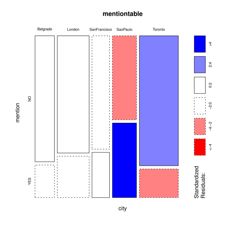
For São Paulo and Toronto the number of messages with mention and NO mention appear to be more than 2.4 standard deviations away from the expected values. The São Paulo chat-room has more people mentioning other people than expected, and for Toronto there are less people mentioning other people than expected.
That’s interesting. A next step would be to explore the sources of these differences. Maybe it’s because of the number of people in each chat-room? Or maybe they already know each other, so they have more one on one conversations?
In conclusion
In Inferential Statistics we deduce properties of an underlying probability distribution. When you have a categorical variable you can use the chi-square test to find the probability of the distribution being the same for two or more populations (or subgroups of a population).
And the steps to use a statistical hypothesis test are:
- First assume the null hypothesis is true
- Then try to prove that it’s impossible that it can be true
- Then if we see that indeed, this probably can’t be true for the results we got, we reject the null hypothesis (or otherwise we fail to reject and accept that the data supports the experimental hypothesis)
Besides that, we also saw that Spacy.Matcher is a great way to extract information from text. Here we did the experiment with mentions from each message but the code has other extracted patterns we could explore.
And that’s it! Thanks for reading!