

According to the Oxford English Dictionary, "greedy" means having excessive desire for something without considering the effect or damage done.
In computer science, a greedy algorithm is an algorithm that finds a solution to problems in the shortest time possible. It picks the path that seems optimal at the moment without regard for the overall optimization of the solution that would be formed.
Edsger Dijkstra, a computer scientist and mathematician who wanted to calculate a minimum spanning tree, introduced the term "Greedy algorithm". Prim and Kruskal came up with optimization techniques for minimizing cost of graphs.
Many Greedy algorithms were developed to solve graph problems. A graph is a structure made up of edges and vertices.
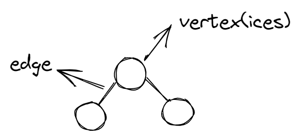
Diagram of a simple graph
Greedy vs Not Greedy Algorithms
An algorithm is greedy when the path picked is regarded as the best option based on a specific criterion without considering future consequences. But it typically evaluates feasibility before making a final decision. The correctness of the solution depends on the problem and criteria used.
Example: A graph has various weights and you are to determine the maximum value in the tree. You'd start by searching each node and checking its weight to see if it is the largest value.
There are two approaches to solving this problem: greedy approach or not greedy.
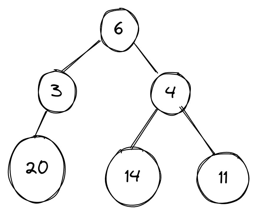
Example graph
This graph consists of different weights and we need to find the maximum value. We'll apply the two approaches on the graph to get the solution.
Greedy Approach
In the images below, a graph has different numbers in its vertices and the algorithm is meant to select the vertex with the largest number.
Starting from vertex 6, then it's faced with two decisions – which is bigger, 3 or 4? The algorithm picks 4, and then is faced with another decision – which is bigger, 14 or 11. It selects 14, and the algorithm ends.
On the other hand there is a vertex labeled 20 but it is attached to vertex 3 which greedy does not consider as the best choice. It is important to select appropriate criteria for making each immediate decision.
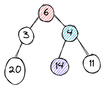
The sample graph showing the greedy approach
Not Greedy Approach
The “not greedy” approach checks all options before arriving at a final solution, unlike the "greedy approach" which stops once it gets its results.
Starting from vertex 6, then it's faced with two decisions – which is bigger, 3 or 4? The algorithm picks 4, and then is faced with another decision – which is bigger, 14 or 11. It selects 14 and keeps it aside.
Then it runs the process again, starting from vertex 6. It selects the vertex with 3 and checks it. 20 is attached to the vertex 3 and the process stops. Now it compares the two results – 20 and 14. 20 is bigger, so it selects the vertex (3) that carries the largest number and the process ends.
This approach considers many possibilities in finding the better solution.
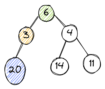
The sample graph showing the non-greedy approach
Characteristics of a Greedy Algorithm
The algorithm solves its problem by finding an optimal solution. This solution can be a maximum or minimum value. It makes choices based on the best option available.
The algorithm is fast and efficient with time complexity of O(n log n) or O(n). Therefore applied in solving large-scale problems.
The search for optimal solution is done without repetition – the algorithm runs once.
It is straightforward and easy to implement.
How to Use Greedy Algorithms
Before applying a greedy algorithm to a problem, you need to ask two questions:
Do you need the best option at the moment from the problem?
Do you need an optimal solution (either minimum or maximum value)?
If your answer to these questions is "Yes", then a greedy algorithm is a good choice to solve your problem.
Procedure
Let’s assume you have a problem with a set of numbers and you need to find the minimum value.
You start of by defining the constraint, which in this case is finding the minimum value. Then each number will be scanned and checked on each constraint which serves as a condition to be fulfilled. If the condition is true, the number(s) is selected and returned as the final solution.
Here's a flowchart representation of this process:
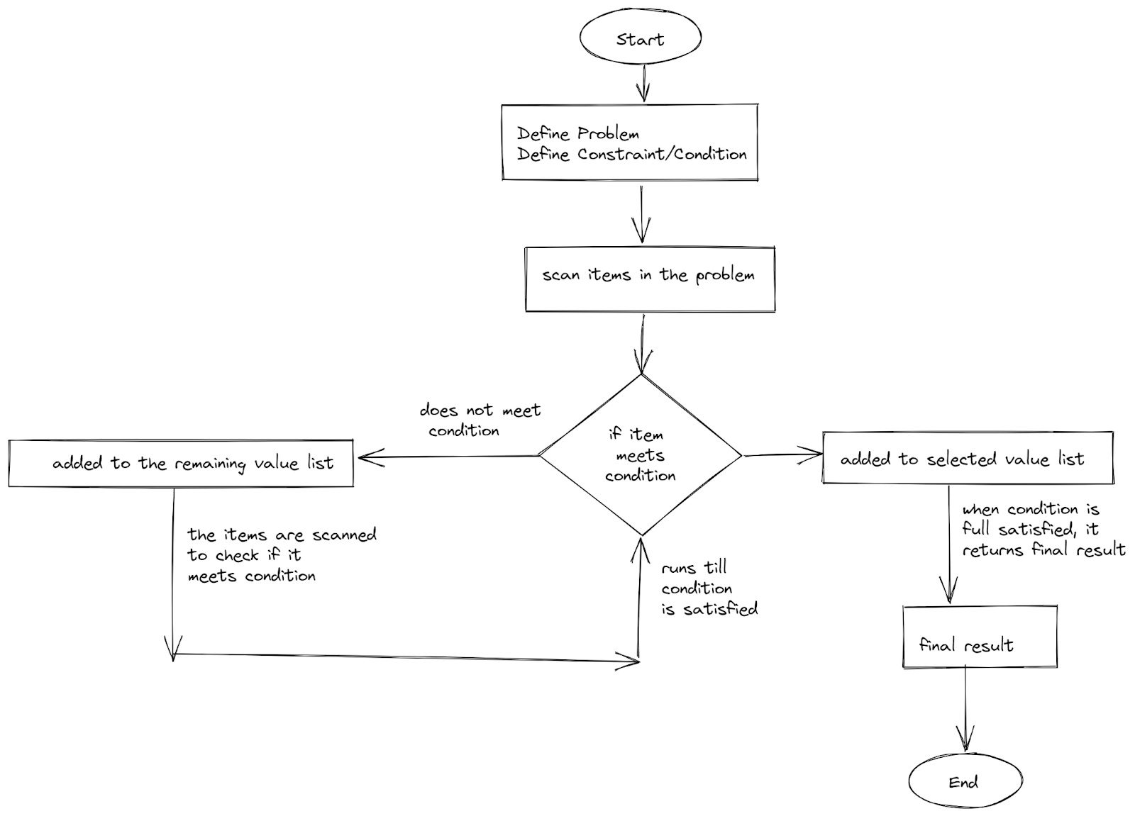
Flow chart showing the process for solving a problem using greedy algorithms
Greedy Algorithm Examples
Problem 1 : Activity Selection Problem
This problem contains a set of activities or tasks that need to be completed. Each one has a start and finish time. The algorithm finds the maximum number of activities that can be done in a given time without them overlapping.
Approach to the Problem
We have a list of activities. Each has a start time and finish time.
First, we sort the activities and start time in ascending order using the finish time of each.
Then we start by picking the first activity. We create a new list to store the selected activity.
To choose the next activity, we compare the finish time of the last activity to the start time of the next activity. If the start time of the next activity is greater than the finish time of the last activity, it can be selected. If not we skip this and check the next one.
This process is repeated until all activities are checked. The final solution is a list containing the activities that can be done.
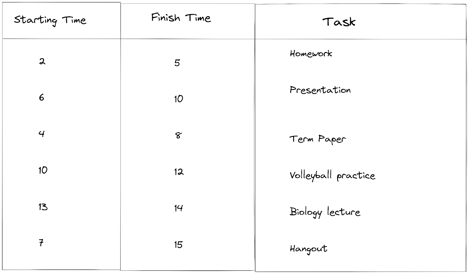
The table below shows a list of activities as well as starting and finish times.
The first step is to sort the finish time in ascending order and arrange the activities with respect to the result.
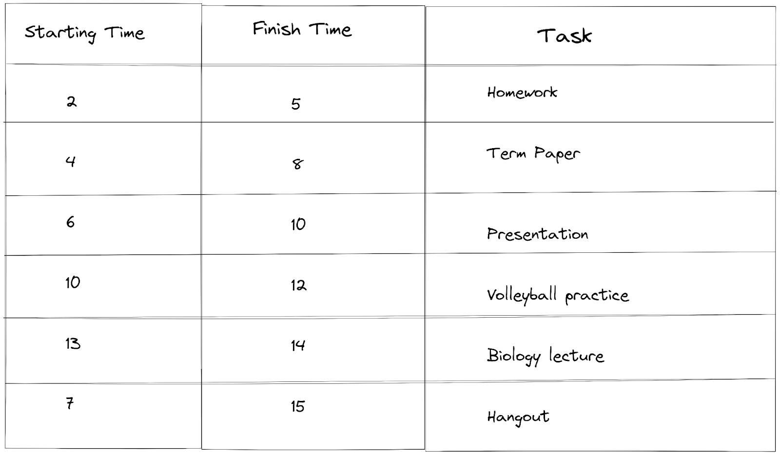
After sorting the activities, we select the first activity and store it in the selected activity list. In our example, the first activity is “Homework”.
Moving to the next activity, we check the finish time of “Homework” (5) which was the last activity selected and the starting time of “Term paper” (4). To pick an activity, the starting time of the next activity must be greater than or equal to the finish time. (4) is less than (5), so we skip the activity and move to the next.
The next activity “Presentation” has a starting time of (6) and it is greater than the finish time (5) of “Homework”. So we select it and add it to our list of selected activities.
For the next activity, we do the same checking. Finish time of “Presentation” is (10), starting time of “Volleyball practice ” is (10). We see that the starting time is equal to the finish time which satisfies one of the conditions, so we select it and add it to our list of selected activities.
Continuing to the next activity, the finish time of “Volleyball” practice is (12) and the starting time of “Biology lecture” is (13). We see the starting time is greater than the finish time so we select it.
For our last activity, the starting time for “Hangout” is (7) and the finishing time of our last activity “Biology lecture” is (14), 7 is less than 14, so we cannot select the activity. Since we are at the end of our activity list, the process ends.
Our final result is the list of selected activities that we can do without time overlapping: {Homework, Presentation, Volleyball practice, Biology lecture}.
Code Implementation of the Example
The variable <data> stores the starting times of each activity, the finish time of each activity, and the list of tasks (or activities) to be performed.
The variable <selected_activity> is an empty list that will store the selected activities that can be performed.
<start_position> shows the position the first activity which is index “0”. This will be our starting point.
data = {
  "start_time": [2 , 6 , 4 , 10 , 13 , 7],
  "finish_time": [5 , 10 , 8 , 12 , 14 , 15],
  "activity": ["Homework" , "Presentation" , "Term paper" , "Volleyball practice" , "Biology lecture" , "Hangout"]
}

selected_activity =[]
start_position = 0
Here's a dataframe table showing the original data:
Original Info

   start_time  finish_time             activity
0           2            5             Homework
1           6           10         Presentation
2           4            8           Term paper
3          10           12  Volleyball practice
4          13           14      Biology lecture
5           7           15              Hangout
Then we sort the finish time in ascending order and rearrange the start time and activity in respect to it. We target the variables by using the keys in the dictionary.
tem = 0
for i in range(0 , len(data['finish_time'])):
   for j in range(0 , len(data['finish_time'])):
       if data['finish_time'][i] < data['finish_time'][j]:
           tem = data['activity'][i] , data['finish_time'][i] , data['start_time'][i]
           data['activity'][i] , data['finish_time'][i] , data['start_time'][i] = data['activity'][j] , data['finish_time'][j] , data['start_time'][j]
           data['activity'][j] , data['finish_time'][j] , data['start_time'][j] = tem
In the code above, we intialized <tem> to zero. We are not using the inbuilt method to sort the finish time. We are using two loops to arrange it in ascending order. <i> and <j> represent the indexes and check if values of the <data['finish_time'][i]> is less than <data['finish_time'][j]>.
If the condition is true, <tem> stores the values of the elements in the <i> position and swaps the corresponding element.
Now we print the final result, here's what we get:
print("Start time: " , data['start_time'])
print("Finish time: " , data['finish_time'])
print("Activity: " , data['activity'])

# Results before sorting
# Start time:  [2, 6, 4, 10, 13, 7]
# Finish time:  [5, 10, 8, 12, 14, 15]
# Activity:  ['Homework', 'Presentation', 'Term paper', 'Volleyball practice', 'Biology lecture', 'Hangout']


# Results after sorting
# Start time:  [2, 4, 6, 10, 13, 7]
# Finish time:  [5, 8, 10, 12, 14, 15]
# Activity:  ['Homework', 'Term paper', 'Presentation', 'Volleyball practice', 'Biology lecture', 'Hangout']
And here's a dataframe table showing the sorted data:
Sorted Info with respect to finish_time

   start_time  finish_time             activity
0       2            5             Homework
1       4            8           Term paper
2       6           10         Presentation
3          10           12       Volleyball practice
4          13           14         Biology lecture
5       7           15          Hangout
After sorting the activities, we start by selecting the first activity, which is “Homework”. It has a starting index of “0” so we use the <start_position> to target the activity and append it to the empty list.
selected_activity.append(data['activity'][start_position])
The condition for selecting an activity is that the start time of the next activity selected is greater than the finish time of the previous activity. If the condition is true, the selected activity is added to the <selected_activity> list.
for pos in range(len(data['finish_time'])):
   if data['start_time'][pos] >= data['finish_time'][start_position]:
       selected_activity.append(data['activity'][pos])
       start_position = pos

print(f"The student can work on the following activities: {selected_activity}")

# Results
# The student can work on the following activities: ['Homework', 'Presentation', 'Volleyball practice', 'Biology lecture']
Here's what it looks like all together:
data = {
  "start_time": [2 , 6 , 4 , 10 , 13 , 7],
  "finish_time": [5 , 10 , 8 , 12 , 14 , 15],
  "activity": ["Homework" , "Presentation" , "Term paper" , "Volleyball practice" , "Biology lecture" , "Hangout"]
}

selected_activity =[]
start_position = 0
# sorting the items in ascending order with respect to finish time
tem = 0
for i in range(0 , len(data['finish_time'])):
   for j in range(0 , len(data['finish_time'])):
       if data['finish_time'][i] < data['finish_time'][j]:
           tem = data['activity'][i] , data['finish_time'][i] , data['start_time'][i]
           data['activity'][i] , data['finish_time'][i] , data['start_time'][i] = data['activity'][j] , data['finish_time'][j] , data['start_time'][j]
           data['activity'][j] , data['finish_time'][j] , data['start_time'][j] = tem

# by default, the first activity is inserted in the list of activities to be selected.

selected_activity.append(data['activity'][start_position])
for pos in range(len(data['finish_time'])):
   if data['start_time'][pos] >= data['finish_time'][start_position]:
       selected_activity.append(data['activity'][pos])
       start_position = pos

print(f"The student can work on the following activities: {selected_activity}")
# Results
# The student can work on the following activities: ['Homework', 'Presentation', 'Volleyball practice', 'Biology lecture']
Problem 2: Fractional Knapsack Problem
A knapsack has a maximum weight, and it can only accommodate a certain set of items. These items have a weight and a value.
The aim is to fill the knapsack with the items that have the highest total values and do not exceed the maximum weight capacity.
Approach to the Problem
There are two elements to consider: the knapsack and the items. The knapsack has a maximum weight and carries some items with a high value.
Scenario: In a jewelry store, there are items made of gold, silver, and wood. The costliest item is gold followed by silver and then wood. If a jewerly thief comes to the store, they take gold because they will make the most profit.
The thief has a bag (knapsack) that they can put those items in. But there is a limit to what the thief can carry because these items can get heavy. The idea is to pick the item the makes the highest profit and fits in the bag (knapsack) without exceeding its maximum weight.
The first step is to find the value to weight ratio of all items to know what fraction each one occupies.
We then sort these ratios in descending order (from highest to lowest ). This way we can pick the ratios with the highest number first knowing that we will make a profit.
When we pick the highest ratio, we find the corresponding weight and add it to the knapsack. There are conditions to be checked.
Condition 1: If the item added has a lesser weight than the maximum weight of the knapsack, more items are added until the sum of all the items in the bag are the same as the maximum weight of the knapsack.
Condition 2: If the sum of the items’ weight in the bag is more than the maximum capacity of the knapsack, we find the fraction of the last item added. To find the fraction, we do the following:
We find the sum of the remaining weights of the items in the knapsack. They must be less than the maximum capacity.
We find the difference between the maximum capacity of the knapsack and the sum of the remaining weights of the items and divide by the weight of the last item to be added.
Fraction = (maximum capacity of the knapsack - sum of remaining weights) / weight of last item to be added
To add the weight of the last item to the knapsack, we multiply the fraction by the weight.
Weight_added = weight of last item to be added * fraction
When we sum up the weights of all the items it will be equal to the knapsack's maximum weight.
Practical Example:
Let's say that the maximum capacity of the knapsack is 17, and there are three items available. The first item is gold, the second item is silver, and third item is wood.
Weight of gold is 10, the weight of silver is 6, and the weight of wood is 2
the value (profit) of gold is 40, the value (profit) of silver is 30, and the value (profit) of wood is 6.
Ratio of gold= value/weight = 40/10 = 4
Ratio of silver = value/weight=30/6 = 5
Ratio of wood = value/weight = 6/2 = 3
Arranging the ratios in descending: 5, 4, 3.
The largest ratio is 5 and we match it to the corresponding weight “6”. It points to silver.
We put silver in the knapsack first and compare it to the maximum weight which is 17. 6 is less than 17 so we have to add another item. Going back to the ratios, the second largest is “4” and it corresponds to the weight of “10” which points to gold.
Now, we put gold in the knapsack, add the weight of the silver and gold, and compare it with the knapsack weight. (6 + 10 = 16). Checking it against the maximum weight, we see that it is less. So we can take another item. We go back to the list of ratios and take the 3rd largest which is “3” and it corresponds to “2” which points to wood.
When we add wood in the knapsack, the total weight is (6 +10+2 = 18) but that is greater than our maximum weight which is 17. We take out the wood from the knapsack and we are left with gold and silver. The total sum of the two is 16 and the maximum capacity is 17. So we need a weight of 1 to make it equal. Now we apply condition 2 discussed above to find the fraction of wood to fit in the knapsack.
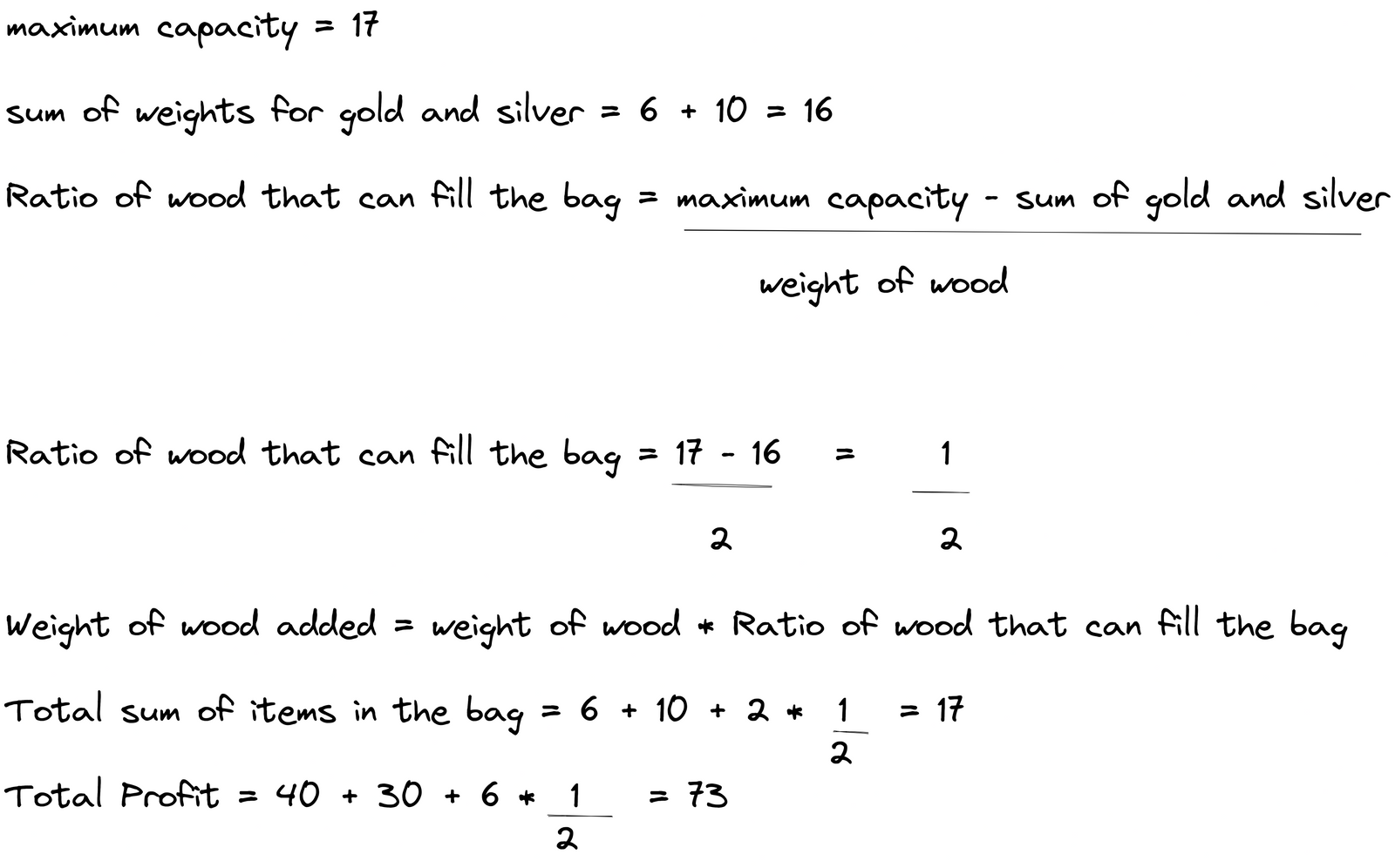
Explanation of filling the remaining space in the backpack with a fractional piece of wood
Now the knapsack is filled.
Code Implementation of the Example
The variable <data> stores the weights of each item and the profits. The variable <maximum_capacity> stores the maximum weight of the knapsack. <selected_wt> is intialized at 0, and it will store the selected weights to be put in the knapsack. Lastly, <max_profit> is intialized as 0, it will store the values of the selected weight.
data = {
    "weight": [10 , 6 , 2],
    "profit":[40 , 30 ,6]
}
max_weight = 17
selected_wt = 0
max_profit = 0
Then we calculate the ratio of the profit to the weight. Ratio = profit/weight:
ratio = [int(data['profit'][i] / data['weight'][i]) for i in range(len(data['profit']))]
Now that we have the ratio, we arrange the elements in descending order, from biggest to smallest. Then the items in weight and profit are arranged according to the positions of the sorted ratio.
for i in range(len(ratio)):
    for j in range(i + 1 , len(ratio)):
        if ratio[i] < ratio[j]:
            ratio[i] , ratio[j] = ratio[j] , ratio[i]
            data['weight'][i] , data['weight'][j] = data['weight'][j] , data['weight'][i]
            data['profit'][i] , data['profit'][j] = data['profit'][j] , data['profit'][i]
After the weight and profit are sorted, we start choosing the items and checking the condition. We loop through the length of ratio to target the index of each item in the list. Note: all items in ratio are arranged from biggest to smallest, so the first item is the maximum value and the last item is the minimum value.
for i in range(len(ratio)):
The first item we select has the highest ratio amongst the rest and it is in index 0. Now that the first weight is selected weight, we check if it is less than maximum weight. If it is, we add items till the total weight is equal to the weight of the knapsack. The second item we select has the second highest ratio amongst the rest and it is in index 1, the arrangement is that order of selection.
For every selected weight, we add it to the selected_wt variable and their corresponding profits to the max_profit variable.
if selected_wt + data['weight'][i] <= max_weight:
          selected_wt += data['weight'][i]
          max_profit += data['profit'][i]
When the sum of the selected weights in the knapsack exceeds the maximum weight, we find the fraction of the weight of the last item added to make the total selected weights be equal to the maximum weight. We do this by finding the difference between the max_weight and the sum of the selected weights divided by the weight of the last item added.
The final profit made from the fraction carried is added to the max_profit variable. Then we return the max_profit as the final result.
      else:
          frac_wt = (max_weight - selected_wt) / data['weight'][i]
          frac_value = data['profit'][i] * frac_wt
          max_profit += frac_value
          selected_wt += (max_weight - selected_wt)
print(max_profit)
Bringing it all together:
data = {
    "weight": [10 , 6 , 2],
    "profit":[40 , 30 ,6]
}
max_weight = 17
selected_wt = 0
max_profit = 0

# finds ratio
ratio = [int(data['profit'][i] / data['weight'][i]) for i in range(len(data['profit']))]

# sort ratio in descending order, rearranges weight and profit in order of the sorted ratio
for i in range(len(ratio)):
    for j in range(i + 1 , len(ratio)):
        if ratio[i] < ratio[j]:
            ratio[i] , ratio[j] = ratio[j] , ratio[i]
            data['weight'][i] , data['weight'][j] = data['weight'][j] , data['weight'][i]
            data['profit'][i] , data['profit'][j] = data['profit'][j] , data['profit'][i]


# checks if selected weight with the highest ratio is less than the maximum weight, if so it adds it to knapsack and stores the profit, select the next item.
# else the sum of the selected weights is more than max weight, finds fraction

for i in range(len(ratio)):
    if selected_wt + data['weight'][i] <= max_weight:
          selected_wt += data['weight'][i]
          max_profit += data['profit'][i]
    else:
          frac_wt = (max_weight - selected_wt) / data['weight'][i]
          frac_value = data['profit'][i] * frac_wt
          max_profit += frac_value
          selected_wt += (max_weight - selected_wt)

print(f"The maximum profit that can be made from each item is: {round(max_profit , 2)} euros")
# Result
# The maximum profit that can be made from each item is: 73.0 euros
Applications of Greedy Algorithms
There are various applications of greedy algorithms. Some of them are:
[Minimum spanning tree](https://en.wikipedia.org/wiki/Minimum_spanning_tree#:~:text=A%20minimum%20spanning%20tree%20(MST,minimum%20possible%20total%20edge%20weight.) is without any cycles and with the minimum possible total edge weight. This tree is derived from a connected undirected graph with weights.
Dijkstra’s shortest path is a search algorithm that finds the shortest path between a vertex and other vertices in a weighted graph.
Travelling salesman problem involves finding the shortest route that visits different places only once and returns to the starting point
Huffman coding assigns shorter code to frequently occurring symbols and longer code to less occurring symbols. It is used to encode data efficiently.
Advantages of Using a Greedy Algorithm
Greedy algorithms are quite straight forward to implement and easy to understand. They are also very efficient and have a lower complexity time of O(N * logN).
They're useful in solving optimization problems, returning a maximum or minimum value.
Disadvantages/Limitations of Using a Greedy Algorithm
Even though greedy algorithms are straightforward and helpful in optimization problems, they don't offer the best solutions at all times.
Also greedy algos only run once, so they don't check the correctness of the result produced.
Conclusion
Greedy algorithms are a straightforward approach to solving optimization problems, returning a minimum or maximum value.
This article explained some examples of greedy algorithms and the approach to tackling each problem. By understanding how a greedy algorithm problems works you can better understand dynamic programming. If you have any questions feel free to reach out to me on Twitter💙.