
By Davis David
Tree-based algorithms are popular machine learning methods used to solve supervised learning problems. These algorithms are flexible and can solve any kind of problem at hand (classification or regression).
Tree-based algorithms tend to use the mean for continuous features or mode for categorical features when making predictions on training samples in the regions they belong to. They also produce predictions with high accuracy, stability, and ease of interpretation.
Examples of Tree-based Algorithms
There are different tree-based algorithms that you can use, such as
- Decision Trees
- Random Forest
- Gradient Boosting
- Bagging (Bootstrap Aggregation)
So every data scientist should learn these algorithms and use them in their machine learning projects.
In this article, you will learn more about the Random forest algorithm. After completing this article, you should be proficient at using the random forest algorithm to solve and build predictive models for classification problems with scikit-learn.
What is Random Forest?
Random forest is one of the most popular tree-based supervised learning algorithms. It is also the most flexible and easy to use.
The algorithm can be used to solve both classification and regression problems. Random forest tends to combine hundreds of decision trees and then trains each decision tree on a different sample of the observations.
The final predictions of the random forest are made by averaging the predictions of each individual tree.
The benefits of random forests are numerous. The individual decision trees tend to overfit to the training data but random forest can mitigate that issue by averaging the prediction results from different trees. This gives random forests a higher predictive accuracy than a single decision tree.
The random forest algorithm can also help you to find features that are important in your dataset. It lies at the base of the Boruta algorithm, which selects important features in a dataset.
Random forest has been used in a variety of applications, for example to provide recommendations of different products to customers in e-commerce.
In medicine, a random forest algorithm can be used to identify the patient’s disease by analyzing the patient’s medical record.
Also in the banking sector, it can be used to easily determine whether the customer is fraudulent or legitimate.
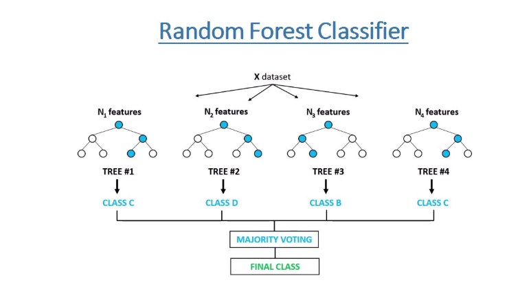
How does the Random Forest algorithm work?
The random forest algorithm works by completing the following steps:
Step 1: The algorithm select random samples from the dataset provided.
Step 2: The algorithm will create a decision tree for each sample selected. Then it will get a prediction result from each decision tree created.
Step 3: Voting will then be performed for every predicted result. For a classification problem, it will use mode, and for a regression problem, it will use mean.
Step 4: And finally, the algorithm will select the most voted prediction result as the final prediction.
 how it works
Random Forest in Practice
Now that you know the ins and outs of the random forest algorithm, let's build a random forest classifier.
We will build a random forest classifier using the Pima Indians Diabetes dataset. The Pima Indians Diabetes Dataset involves predicting the onset of diabetes within 5 years based on provided medical details. This is a binary classification problem.
Our task is to analyze and create a model on the Pima Indian Diabetes dataset to predict if a particular patient is at a risk of developing diabetes, given other independent factors.
We will start by importing important packages that we will use to load the dataset and create a random forest classifier. We will use the scikit-learn library to load and use the random forest algorithm.
# import important packages
import numpy as np
import pandas as pd
import matplotlib.pyplot as plt
import seaborn as sns

%matplotlib inline

from sklearn.model_selection import train_test_split
from sklearn.ensemble import RandomForestClassifier
from sklearn.metrics import accuracy_score
from sklearn.preprocessing import StandardScaler, MinMaxScaler
import pandas_profiling

from matplotlib import rcParams
import warnings

warnings.filterwarnings("ignore")

# figure size in inches
rcParams["figure.figsize"] = 10, 6
np.random.seed(42)
Dataset
Then load the dataset from the data directory:
# Load dataset
data = pd.read_csv("../data/pima_indians_diabetes.csv")
Now we can observe the sample of the dataset.
# show sample of the dataset
data.sample(5)
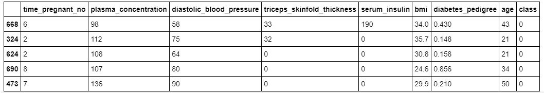
As you can see, in our dataset we have different features with numerical values.
Let's understand the list of features we have in this dataset.
# show columns
data.columns
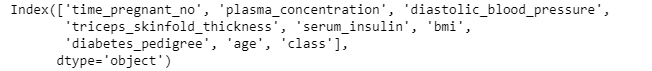
In this dataset, there are 8 input features and 1 output / target feature. Missing values are believed to be encoded with zero values. The meaning of the variable names are as follows (from the first to the last feature):
- Number of times pregnant.
- Plasma glucose concentration a 2 hours in an oral glucose tolerance test.
- Diastolic blood pressure (mm Hg).
- Triceps skinfold thickness (mm).
- 2-hour serum insulin (mu U/ml).
- Body mass index (weight in kg/(height in m)^2).
- Diabetes pedigree function.
- Age (years).
- Class variable (0 or 1).
Then we split the dataset into independent features and target feature. Our target feature for this dataset is called class.
# split data into input and taget variable(s)

X = data.drop("class", axis=1)
y = data["class"]
Preprocessing the Dataset
Before we create a model we need to standardize our independent features by using the standardScaler method from scikit-learn.
# standardize the dataset
scaler = StandardScaler()
X_scaled = scaler.fit_transform(X)
You can learn more on how and why to standardize your data from this article by clicking here.
Splitting the dataset into Training and Test data
We now split our processed dataset into training and test data. The test data will be 10% of the entire processed dataset.
# split into train and test set
X_train, X_test, y_train, y_test = train_test_split(
    X_scaled, y, stratify=y, test_size=0.10, random_state=42
)
Building the Random Forest Classifier
Now is time to create our random forest classifier and then train it on the train set. We will also pass the number of trees (100) in the forest we want to use through the parameter called n_estimators.
# create the classifier
classifier = RandomForestClassifier(n_estimators=100)

# Train the model using the training sets
classifier.fit(X_train, y_train)
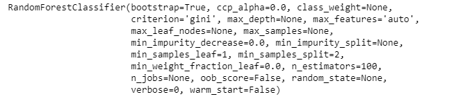
The above output shows different parameter values of the random forest classifier used during the training process on the train data.
After training we can perform prediction on the test data.
# predictin on the test set
y_pred = classifier.predict(X_test)
Then we check the accuracy using actual and predicted values from the test data.
# Calculate Model Accuracy
print("Accuracy:", accuracy_score(y_test, y_pred))
Accuracy: 0.8051948051948052
Our accuracy is around 80.5% which is good. But we can always make it better.
Identify Important Features
As I said before, we can also check the important features by using the featureimportances variable from the random forest algorithm in scikit-learn.
# check Important features
feature_importances_df = pd.DataFrame(
    {"feature": list(X.columns), "importance": classifier.feature_importances_}
).sort_values("importance", ascending=False)

# Display
feature_importances_df
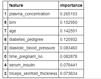 Important Features
The figure above shows the relative importance of features and their contribution to the model. We can also visualize these features and their scores using the seaborn and matplotlib libraries.
# visualize important featuers

# Creating a bar plot
sns.barplot(x=feature_importances_df.feature, y=feature_importances_df.importance)
# Add labels to your

plt.xlabel("Feature Importance Score")
plt.ylabel("Features")
plt.title("Visualizing Important Features")
plt.xticks(
    rotation=45, horizontalalignment="right", fontweight="light", fontsize="x-large"
)
plt.show()
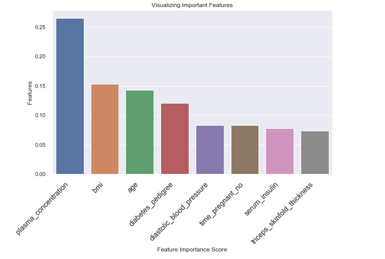
From the figure above, you can see the triceps_skinfold_thickness feature has low importance and does not contribute much to the prediction.
This means that we can remove this feature and train our random forest classifier again and then see if it can improve its performance on the test data.
# load data with selected features
X = data.drop(["class", "triceps_skinfold_thickness"], axis=1)
y = data["class"]

# standardize the dataset
scaler = StandardScaler()
X_scaled = scaler.fit_transform(X)

# split into train and test set
X_train, X_test, y_train, y_test = train_test_split(
    X_scaled, y, stratify=y, test_size=0.10, random_state=42
)
We will train the random forest algorithm with the selected processed features from our dataset, perform predictions, and then find the accuracy of the model.
# Create a Random Classifier
clf = RandomForestClassifier(n_estimators=100)

# Train the model using the training sets
clf.fit(X_train, y_train)

# prediction on test set
y_pred = clf.predict(X_test)

# Calculate Model Accuracy,
print("Accuracy:", accuracy_score(y_test, y_pred))
Accuracy: 0.8181818181818182
Now the model accuracy has increased from 80.5% to 81.8% after we removed the least important feature called _triceps_skinfoldthickness.
This suggests that it is very important to check important features and see if you can remove the least important features to increase your model's performance.
Wrapping up
Tree-based algorithms are really important for every data scientist to learn. In this article, you've learned the basics of tree-based algorithms and how to create a classification model by using the random forest algorithm.
I also recommend you try other types of tree-based algorithms such as the Extra-trees algorithm.
You can download the dataset and notebook used in this article here: https://github.com/Davisy/Random-Forest-classification-Tutorial
Congratulations, you have made it to the end of this article!
If you learned something new or enjoyed reading this article, please share it so that others can see it. Until then, see you in the next post! I can also be reached on Twitter @Davis_McDavid