by Daniel Deutsch

Get started with TensorFlow on law and statistics

• What this is about
• What we will use
• Get started
• Shell commands for installing everything you need
• Get data and draw a plot
• Import everything you need
• Create and plot some numbers
• Build a TensorFlow model
• Prepare data
• Set up variables and operations for TensorFlow
• Start the calculations with a TensorFlow session
• Visualize the result and process

What this is about

As I am exploring TensorFlow, I wanted build a beginner example and document it. This is a very basic example that uses a gradient descent optimization to train parameters with TensorFlow. The key variables are evidence and convictions. It will illustrate:

• how the number of convictions depend upon the number of pieces of evidence
• how to predict the number of convictions using a regression model

The Python file is in my repository on GitHub.

See the article in better formatting on GitHub.

What we will use

1. TensorFlow (as tf)

Tensors

• tf.placeholders
• tf.Variables

Helper function

• tf.global_variables_initializer

Math Operations

• tf.add
• tf.multiply
• tf.reduce_sum
• tf.pow

Building a graph

• tf.train.GradientDescentOptimizer

Session

• tf.Session

2. Numpy (as np)

• np.random.seed
• np.random.zeros
• np.random.randint
• np.random.randn
• np.random.asanyarray

3. Matplotlib

4. Math

Getting started

Install TensorFlow with virtualenv. See the guide on the TF website.

Shell commands for installing everything you need

sudo easy_install pip

pip3 install --upgrade virtualenv

virtualenv --system-site-packages <targetDirectory>

cd <targetDirectory>

source ./bin/activate

easy_install -U pip3

pip3 install tensorflow

pip3 install matplotlib

Get data and draw a plot

Import everything you need

import tensorflow as tfimport numpy as npimport mathimport matplotlibmatplotlib.use('TkAgg')import matplotlib.pyplot as pltimport matplotlib.animation as animation

As you can see I am using the “TkAgg” backend from matplotlib. This allows me to debug with my vsCode and macOS setup without any further complicated installments.

Create and plot some numbers

# Generate evidence numbers between 10 and 20# Generate a number of convictions from the evidence with a random noise addednp.random.seed(42)sampleSize = 200numEvid = np.random.randint(low=10, high=50, size=sampleSize)numConvict = numEvid * 10 + np.random.randint(low=200, high=400, size=sampleSize)

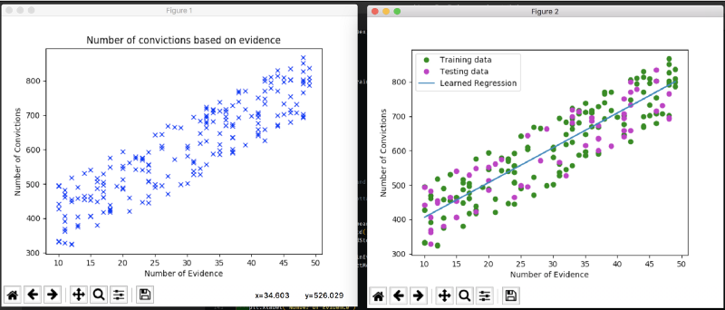
# Plot the data to get a feelingplt.title("Number of convictions based on evidence")plt.plot(numEvid, numConvict, "bx")plt.xlabel("Number of Evidence")plt.ylabel("Number of Convictions")plt.show(block=False)  # Use the keyword 'block' to override the blocking behavior

I am creating random values for the evidence. The number of convictions depends on the amount (number) of evidence, with random noise. Of course those numbers are made up, but they are just used to prove a point.

Build a TensorFlow model

To build a basic machine learning model, we need to prepare the data. Then we make predictions, measure the loss, and optimize by minimizing the loss.

Prepare data

# create a function for normalizing values# use 70% of the data for training (the remaining 30% shall be used for testing)def normalize(array):    return (array - array.mean()) / array.std()

numTrain = math.floor(sampleSize * 0.7)

# convert list to an array and normalize arraystrainEvid = np.asanyarray(numEvid[:numTrain])trainConvict = np.asanyarray(numConvict[:numTrain])trainEvidNorm = normalize(trainEvid)trainConvictdNorm = normalize(trainConvict)

testEvid = np.asanyarray(numEvid[numTrain:])testConvict = np.asanyarray(numConvict[numTrain:])testEvidNorm = normalize(testEvid)testConvictdNorm = normalize(testConvict)

We are splitting the data into training and testing portions. Afterwards, we normalize the values, as this is necessary for machine learning projects. (See also “feature scaling”.)

Set up variables and operations for TensorFlow

# define placeholders  and variablestfEvid = tf.placeholder(tf.float32, name="Evid")tfConvict = tf.placeholder(tf.float32, name="Convict")tfEvidFactor = tf.Variable(np.random.randn(), name="EvidFactor")tfConvictOffset = tf.Variable(np.random.randn(), name="ConvictOffset")

# define the operation for predicting the conviction based on evidence by adding both values# define a loss function (mean squared error)tfPredict = tf.add(tf.multiply(tfEvidFactor, tfEvid), tfConvictOffset)tfCost = tf.reduce_sum(tf.pow(tfPredict - tfConvict, 2)) / (2 * numTrain)

# set a learning rate and a gradient descent optimizerlearningRate = 0.1gradDesc = tf.train.GradientDescentOptimizer(learningRate).minimize(tfCost)

The pragmatic differences between tf.placeholder and tf.Variable are:

• placeholders are allocated storage for data, and initial values are not required
• variables are used for parameters to learn, and initial values are required. The values can be derived from training.

I use the TensorFlow operators precisely as tf.add(…), because it is pretty clear what library is used for the calculation. This is instead of using the + operator.

Start the calculations with a TensorFlow session

# initialize variablesinit = tf.global_variables_initializer()

with tf.Session() as sess:    sess.run(init)

    # set up iteration parameters    displayEvery = 2    numTrainingSteps = 50

    # Calculate the number of lines to animation    # define variables for updating during animation    numPlotsAnim = math.floor(numTrainingSteps / displayEvery)    evidFactorAnim = np.zeros(numPlotsAnim)    convictOffsetAnim = np.zeros(numPlotsAnim)    plotIndex = 0

    # iterate through the training data    for i in range(numTrainingSteps):

        # ======== Start training by running the session and feeding the gradDesc        for (x, y) in zip(trainEvidNorm, trainConvictdNorm):            sess.run(gradDesc, feed_dict={tfEvid: x, tfConvict: y})

        # Print status of learning        if (i + 1) % displayEvery == 0:            cost = sess.run(                tfCost, feed_dict={tfEvid: trainEvidNorm, tfConvict: trainConvictdNorm}            )            print(                "iteration #:",                "%04d" % (i + 1),                "cost=",                "{:.9f}".format(cost),                "evidFactor=",                sess.run(tfEvidFactor),                "convictOffset=",                sess.run(tfConvictOffset),            )

            # store the result of each step in the animation variables            evidFactorAnim[plotIndex] = sess.run(tfEvidFactor)            convictOffsetAnim[plotIndex] = sess.run(tfConvictOffset)            plotIndex += 1

    # log the optimized result    print("Optimized!")    trainingCost = sess.run(        tfCost, feed_dict={tfEvid: trainEvidNorm, tfConvict: trainConvictdNorm}    )    print(        "Trained cost=",        trainingCost,        "evidFactor=",        sess.run(tfEvidFactor),        "convictOffset=",        sess.run(tfConvictOffset),        "\n",    )

Now we come to the actual training and the most interesting part.

The graph is now executed in a tf.Session. I am using "feeding" as it lets you inject data into any Tensor in a computation graph. You can see more on reading data here.

tf.Session() is used to create a session that is automatically closed on exiting the context. The session also closes when an uncaught exception is raised.

The tf.Session.run method is the main mechanism for running a tf.Operation or evaluating a tf.Tensor. You can pass one or more tf.Operation or tf.Tensor objects to tf.Session.run, and TensorFlow will execute the operations that are needed to compute the result.

First, we are running the gradient descent training while feeding it the normalized training data. After that, we are calculating the the loss.

We are repeating this process until the improvements per step are very small. Keep in mind that the tf.Variables (the parameters) have been adapted throughout and now reflect an optimum.

Visualize the result and process

# de-normalize variables to be plotable again    trainEvidMean = trainEvid.mean()    trainEvidStd = trainEvid.std()    trainConvictMean = trainConvict.mean()    trainConvictStd = trainConvict.std()    xNorm = trainEvidNorm * trainEvidStd + trainEvidMean    yNorm = (        sess.run(tfEvidFactor) * trainEvidNorm + sess.run(tfConvictOffset)    ) * trainConvictStd + trainConvictMean

    # Plot the result graph    plt.figure()

    plt.xlabel("Number of Evidence")    plt.ylabel("Number of Convictions")

    plt.plot(trainEvid, trainConvict, "go", label="Training data")    plt.plot(testEvid, testConvict, "mo", label="Testing data")    plt.plot(xNorm, yNorm, label="Learned Regression")    plt.legend(loc="upper left")

    plt.show()

    # Plot an animated graph that shows the process of optimization    fig, ax = plt.subplots()    line, = ax.plot(numEvid, numConvict)

    plt.rcParams["figure.figsize"] = (10, 8) # adding fixed size parameters to keep animation in scale    plt.title("Gradient Descent Fitting Regression Line")    plt.xlabel("Number of Evidence")    plt.ylabel("Number of Convictions")    plt.plot(trainEvid, trainConvict, "go", label="Training data")    plt.plot(testEvid, testConvict, "mo", label="Testing data")

    # define an animation function that changes the ydata    def animate(i):        line.set_xdata(xNorm)        line.set_ydata(            (evidFactorAnim[i] * trainEvidNorm + convictOffsetAnim[i]) * trainConvictStd            + trainConvictMean        )        return (line,)

    # Initialize the animation with zeros for y    def initAnim():        line.set_ydata(np.zeros(shape=numConvict.shape[0]))        return (line,)

    # call the animation    ani = animation.FuncAnimation(        fig,        animate,        frames=np.arange(0, plotIndex),        init_func=initAnim,        interval=200,        blit=True,    )

    plt.show()

To visualize the process, it is helpful to plot the result and maybe even the optimization process.

Check out this Pluralsight course which helped me a lot to get started. :)

Thanks for reading my article! Feel free to leave any feedback!

Daniel is a LL.M. student in business law, working as a software engineer and organizer of tech related events in Vienna. His current personal learning efforts focus on machine learning.

Connect on:

• LinkedIn
• Github
• Medium
• Twitter
• Steemit
• Hashnode