
By Sachin Malhotra
by Sachin Malhotra and Divya Godayal
Welcome back, Caretaker!
In case you’ve forgotten the problem we were trying to tackle in the previous article, let us revise it for you.
So there’s this naughty kid Peter and he’s going to pester his new caretaker, you!
As a caretaker, one of the most important tasks for you is to tuck Peter in bed and make sure he is sound asleep. Once you’ve tucked him in, you want to make sure that he’s actually asleep and not up to some mischief.
You cannot, however, enter the room again, as that would surely wake Peter up. All you can hear are the noises that might come from the room.
Either the room is quiet or there is noise coming from the room. These are your observations.
All you have as the caretaker are:
- a set of observations, which is basically a sequence containing noise or quiet over time, and
- A state diagram provided by Peter’s mom — who happens to be a neurological scientist — that contains all the different sets of probabilities that you can use to solve the problem defined below.
The problem
Given the state diagram and a sequence of N observations over time, we need to tell the state of the baby at the current point in time. Mathematically, we have N observations over times t0, t1, t2 .... tN . We want to find out if Peter would be awake or asleep, or rather which state is more probable at time tN+1 .
In case any of this seems like Greek to you, go read the previous article to brush up on the Markov Chain Model, Hidden Markov Models, and Part of Speech Tagging.
In that previous article, we had briefly modeled the problem of Part of Speech tagging using the Hidden Markov Model.
The problem of Peter being asleep or not is just an example problem taken up for a better understanding of some of the core concepts involved in these two articles. At the core, the articles deal with solving the Part of Speech tagging problem using the Hidden Markov Models.
So, before moving on to the Viterbi Algorithm, let’s first look at a much more detailed explanation of how the tagging problem can be modeled using HMMs.
Generative Models and the Noisy Channel Model
A lot of problems in Natural Language Processing are solved using a supervised learning approach.
Supervised problems in machine learning are defined as follows. We assume training examples (x(1), y(1)). . .(x(m) , y(m)), where each example consists of an input x(i) paired with a label y(i) . We use X to refer to the set of possible inputs, and Y to refer to the set of possible labels. Our task is to learn a function f : X → Y that maps any input x to a label f(x).
In tagging problems, each x(i) would be a sequence of words X1 X2 X3 …. Xn(i), and each y(i) would be a sequence of tags Y1 Y2 Y3 … Yn(i)(we use n(i)to refer to the length of the i’th training example). X would refer to the set of all sequences x1 . . . xn, and Y would be the set of all tag sequences y1 . . . yn. Our task would be to learn a function f : X → Y that maps sentences to tag sequences.
An intuitive approach to get an estimate for this problem is to use conditional probabilities. p(y | x) which is the probability of the output y given an input x. The parameters of the model would be estimated using the training samples. Finally, given an unknown input x we would like to find
f(x) = arg max(p(y | x)) ∀y ∊ Y
This here is the conditional model to solve this generic problem given the training data. Another approach that is mostly adopted in machine learning and natural language processing is to use a generative model.
Rather than directly estimating the conditional distribution p(y|x), in generative models we instead model the joint probability p(x, y) over all the (x, y) pairs.
We can further decompose the joint probability into simpler values using Bayes’ rule:
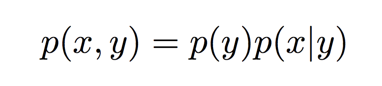
p(y)is the prior probability of any input belonging to the label y.p(x | y)is the conditional probability of input x given the label y.
We can use this decomposition and the Bayes rule to determine the conditional probability.
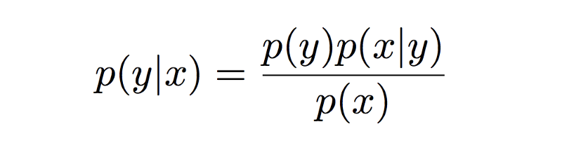
Remember, we wanted to estimate the function
f(x) = arg max( p(y|x) ) ∀y ∊ Y
f(x) = arg max( p(y) * p(x | y) )
The reason we skipped the denominator here is because the probability p(x) remains the same no matter what the output label being considered. And so, from a computational perspective, it is treated as a normalization constant and is normally ignored.
Models that decompose a joint probability into terms p(y) and p(x|y) are often called noisy-channel models. Intuitively, when we see a test example x, we assume that it has been generated in two steps:
- first, a label y has been chosen with probability p(y)
- second, the example x has been generated from the distribution p(x|y). The model p(x|y) can be interpreted as a “channel” which takes a label y as its input, and corrupts it to produce x as its output.
Generative Part of Speech Tagging Model
Let us assume a finite set of words V and a finite sequence of tags K. Then the set S will be the set of all sequence, tags pairs <x1, x2, x3 ... xn, y1, y2, y3, ..., yn> such that n > 0 ∀x ∊ V and ∀y ∊ K .
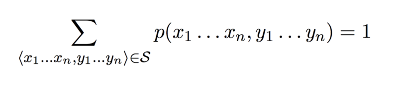
A generative tagging model is then the one where
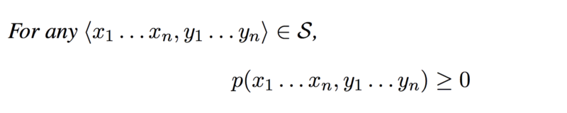
2.
Given a generative tagging model, the function that we talked about earlier from input to output becomes
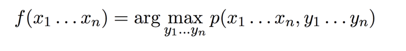
Thus for any given input sequence of words, the output is the highest probability tag sequence from the model. Having defined the generative model, we need to figure out three different things:
- How exactly do we define the generative model probability
p(<x1, x2, x3 ... xn, y1, y2, y3, ..., yn>) - How do we estimate the parameters of the model, and
- How do we efficiently calculate

Let us look at how we can answer these three questions side by side, once for our example problem and then for the actual problem at hand: part of speech tagging.
Defining the Generative Model
Let us first look at how we can estimate the probability p(x1 .. xn, y1 .. yn) using the HMM.
We can have any N-gram HMM which considers events in the previous window of size N.
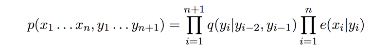
The formulas provided hereafter are corresponding to a Trigram Hidden Markov Model.
Trigram Hidden Markov Model
A trigram Hidden Markov Model can be defined using
- A finite set of states.
- A sequence of observations.
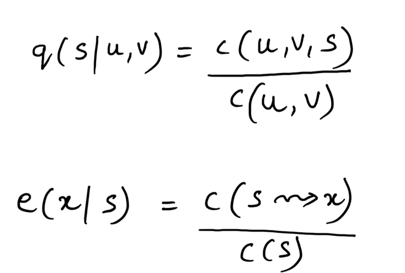
- q(s|u, v)
Transition probability defined as the probability of a state “s” appearing right after observing “u” and “v” in the sequence of observations. - e(x|s)
Emission probability defined as the probability of making an observation x given that the state was s.
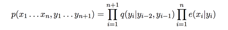
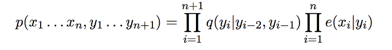
Then, the generative model probability would be estimated as
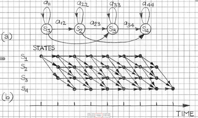
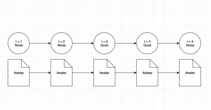
As for the baby sleeping problem that we are considering, we will have only two possible states: that the baby is either awake or he is asleep. The caretaker can make only two observations over time. Either there is noise coming in from the room or the room is absolutely quiet. The sequence of observations and states can be represented as follows:
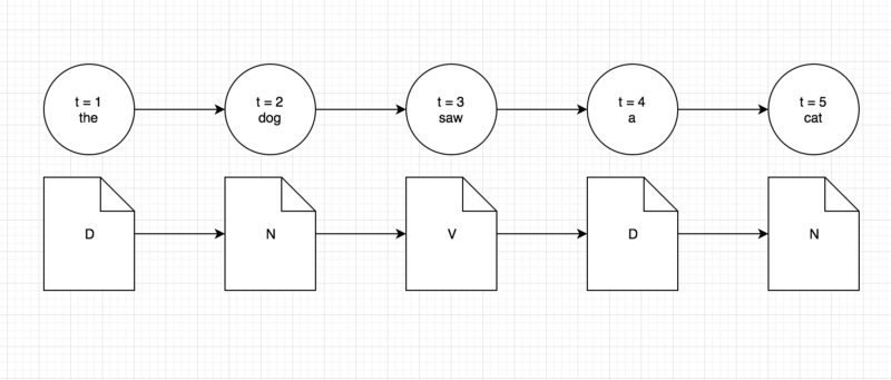
Coming on to the part of speech tagging problem, the states would be represented by the actual tags assigned to the words. The words would be our observations. The reason we say that the tags are our states is because in a Hidden Markov Model, the states are always hidden and all we have are the set of observations that are visible to us. Along similar lines, the sequence of states and observations for the part of speech tagging problem would be
Estimating the model’s parameters
We will assume that we have access to some training data. The training data consists of a set of examples where each example is a sequence consisting of the observations, every observation being associated with a state. Given this data, how do we estimate the parameters of the model?
Estimating the model’s parameters is done by reading various counts off of the training corpus we have, and then computing maximum likelihood estimates:
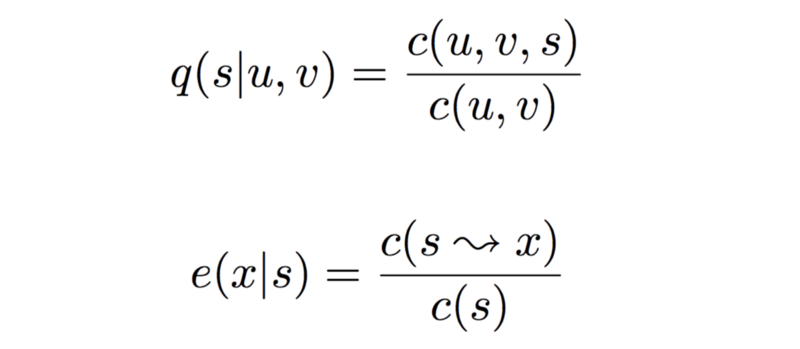
We already know that the first term represents transition probability and the second term represents the emission probability. Let us look at what the four different counts mean in the terms above.
- c(u, v, s) represents the trigram count of states u, v and s. Meaning it represents the number of times the three states u, v and s occurred together in that order in the training corpus.
- c(u, v) following along similar lines as that of the trigram count, this is the bigram count of states u and v given the training corpus.
- c(s → x) is the number of times in the training set that the state s and observation x are paired with each other. And finally,
- c(s) is the prior probability of an observation being labelled as the state s.
Let us look at a sample training set for the toy problem first and see the calculations for transition and emission probabilities using the same.
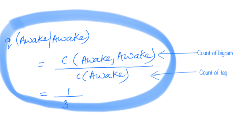
The BLUE markings represent the transition probability, and RED is for emission probability calculations.
Note that since the example problem only has two distinct states and two distinct observations, and given that the training set is very small, the calculations shown below for the example problem are using a bigram HMM instead of a trigram HMM.
Peter’s mother was maintaining a record of observations and states. And thus she even provided you with a training corpus to help you get the transition and emission probabilities.
Transition Probability Example:

Emission Probability Example:

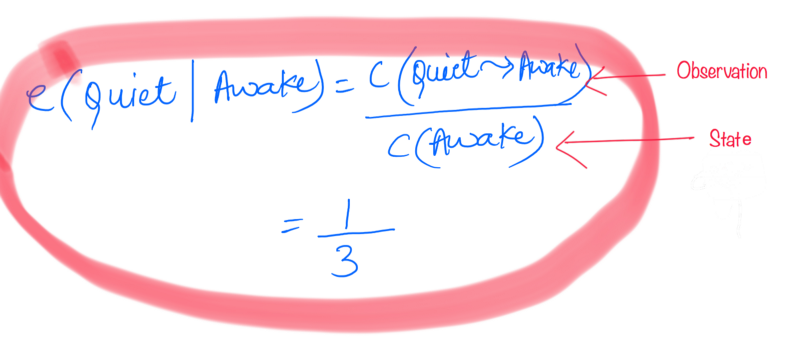
That was quite simple, since the training set was very small. Let us look at a sample training set for our actual problem of part of speech tagging. Here we can consider a trigram HMM, and we will show the calculations accordingly.
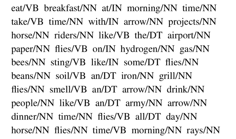
We will use the following sentences as a corpus of training data (the notation word/TAG means word tagged with a specific part-of-speech tag).
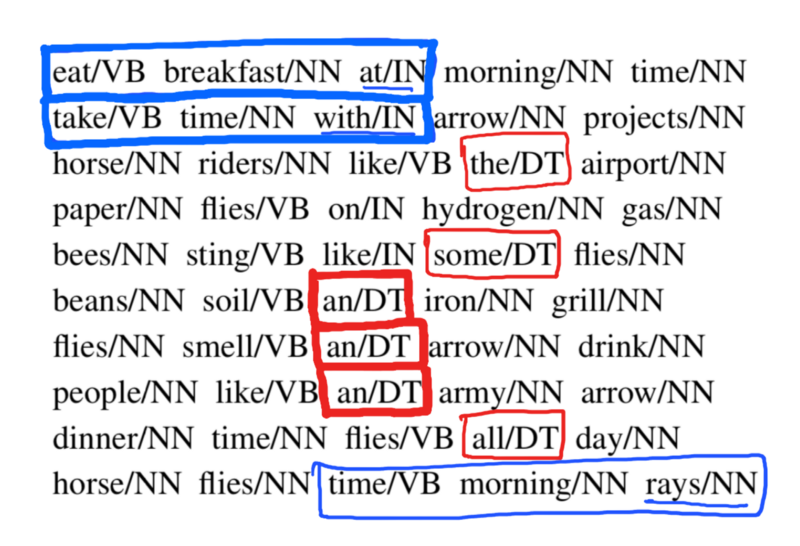
The training set that we have is a tagged corpus of sentences. Every sentence consists of words tagged with their corresponding part of speech tags. eg:- eat/VB means that the word is “eat” and the part of speech tag in this sentence in this very context is “VB” i.e. Verb Phrase. Let us look at a sample calculation for transition probability and emission probability just like we saw for the baby sleeping problem.
Transition Probability
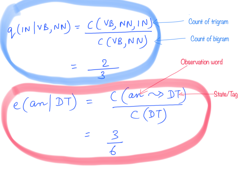
Let’s say we want to calculate the transition probability q(IN | VB, NN). For this, we see how many times we see a trigram (VB,NN,IN) in the training corpus in that specific order. We then divide it by the total number of times we see the bigram (VB,NN) in the corpus.
Emission Probability
Let’s say we want to find out the emission probability e(an | DT). For this, we see how many times the word “an” is tagged as “DT” in the corpus and divide it by the total number of times we see the tag “DT” in the corpus.
So if you look at these calculations, it shows that calculating the model’s parameters is not computationally expensive. That is, we don’t have to do multiple passes over the training data to calculate these parameters. All we need are a bunch of different counts, and a single pass over the training corpus should provide us with that.
Let’s move on and look at the final step that we need to look at given a generative model. That step is efficiently calculating

We will be looking at the famous Viterbi Algorithm for this calculation.
Finding the most probable sequence — Viterbi Algorithm
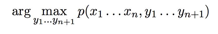
Finally, we are going to solve the problem of finding the most likely sequence of labels given a set of observations x1 … xn. That is, we are to find out
The probability here is expressed in terms of the transition and emission probabilities that we learned how to calculate in the previous section of the article. Just to remind you, the formula for the probability of a sequence of labels given a sequence of observations over “n” time steps is
Before looking at an optimized algorithm to solve this problem, let us first look at a simple brute force approach to this problem. Basically, we need to find out the most probable label sequence given a set of observations out of a finite set of possible sequences of labels. Let’s look at the total possible number of sequences for a small example for our example problem and also for a part of speech tagging problem.
Say we have the following set of observations for the example problem.
Noise Quiet Noise
We have two possible labels {Asleep and Awake}. Some of the possible sequence of labels for the observations above are:
Awake Awake Awake
Awake Awake Asleep
Awake Asleep Awake
Awake Asleep Asleep
In all we can have 2³ = 8 possible sequences. This might not seem like very many, but if we increase the number of observations over time, the number of sequences would increase exponentially. This is the case when we only had two possible labels. What if we have more? As is the case with part of speech tagging.
For example, consider the sentence
the dog barks
and assuming that the set of possible tags are {D, N, V}, let us look at some of the possible tag sequences:
D D DD D ND D VD N DD N ND N V ... etc
Here, we would have 3³ = 27 possible tag sequences. And as you can see, the sentence was extremely short and the number of tags weren’t very many. In practice, we can have sentences that might be much larger than just three words. Then the number of unique labels at our disposal would also be too high to follow this enumeration approach and find the best possible tag sequence this way.
So the exponential growth in the number of sequences implies that for any reasonable length sentence, the brute force approach would not work out as it would take too much time to execute.
Instead of this brute force approach, we will see that we can find the highest probable tag sequence efficiently using a dynamic programming algorithm known as the Viterbi Algorithm.
Let us first define some terms that would be useful in defining the algorithm itself. We already know that the probability of a label sequence given a set of observations can be defined in terms of the transition probability and the emission probability. Mathematically, it is
Let us look at a truncated version of this which is
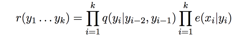
and let us call this the cost of a sequence of length k.
So the definition of “r” is simply considering the first k terms off of the definition of probability where k ∊ {1..n} and for any label sequence y1…yk.
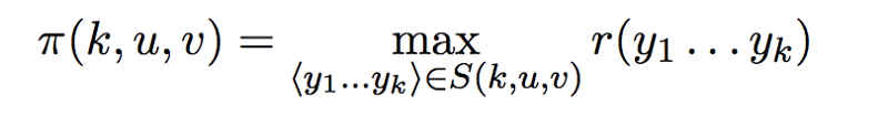
Next we have the set S(k, u, v) which is basically the set of all label sequences of length k that end with the bigram (u, v) i.e.
Finally, we define the term π(k, u, v) which is basically the sequence with the maximum cost.
The main idea behind the Viterbi Algorithm is that we can calculate the values of the term π(k, u, v) efficiently in a recursive, memoized fashion. In order to define the algorithm recursively, let us look at the base cases for the recursion.
π(0, *, *) = 1
π(0, u, v) = 0
Since we are considering a trigram HMM, we would be considering all of the trigrams as a part of the execution of the Viterbi Algorithm.
Now, we can start the first trigram window from the first three words of the sentence but then the model would miss out on those trigrams where the first word or the first two words occurred independently. For that reason, we consider two special start symbols as * and so our sentence becomes
* * x1 x2 x3 ...... xn
And the first trigram we consider then would be (, , x1) and the second one would be (*, x1, x2).
Now that we have all our terms in place, we can finally look at the recursive definition of the algorithm which is basically the heart of the algorithm.
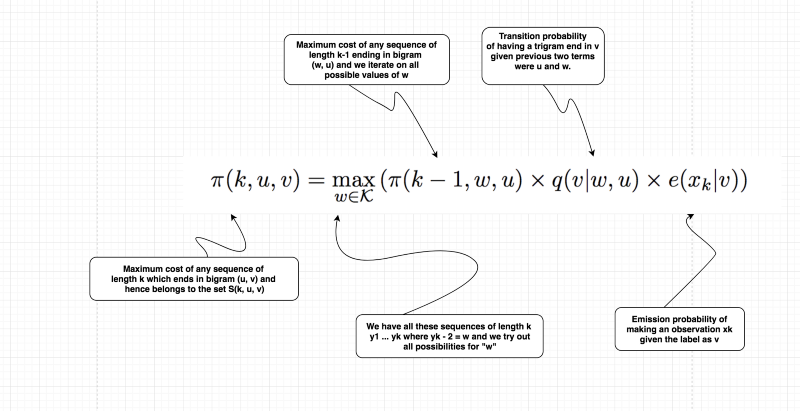
This definition is clearly recursive, because we are trying to calculate one π term and we are using another one with a lower value of k in the recurrence relation for it.

Every sequence would end with a special STOP symbol. For the trigram model, we would also have two special start symbols “*” in the beginning.
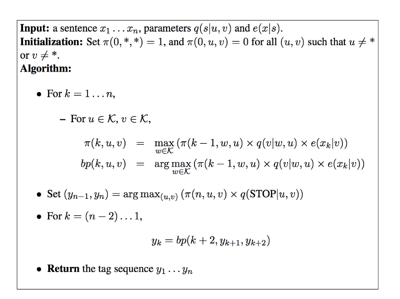
Have a look at the pseudo-code for the entire algorithm.
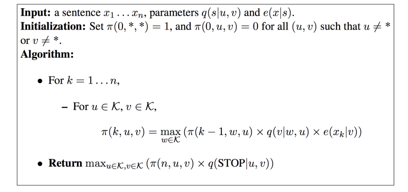
The algorithm first fills in the π(k, u, v) values in using the recursive
definition. It then uses the identity described before to calculate the highest probability for any sequence.
The running time for the algorithm is O(n|K|³), hence it is linear in the length of the sequence, and cubic in the number of tags.
NOTE: We would be showing calculations for the baby sleeping problem and the part of speech tagging problem based off a bigram HMM only. The calculations for the trigram are left to the reader to do themselves. But the code that is attached at the end of this article is based on a trigram HMM. It’s just that the calculations are easier to explain and portray for the Viterbi algorithm when considering a bigram HMM instead of a trigram HMM.
Therefore, before showing the calculations for the Viterbi Algorithm, let us look at the recursive formula based on a bigram HMM.
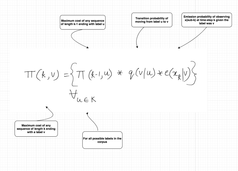
This one is extremely similar to the one we saw before for the trigram model, except that now we are only concerning ourselves with the current label and the one before, instead of two before. The complexity of the algorithm now becomes O(n|K|²).
Calculations for Baby Sleeping Problem
Now that we have the recursive formula ready for the Viterbi Algorithm, let us see a sample calculation of the same firstly for the example problem that we had, that is, the baby sleeping problem, and then for the part of speech tagging version.
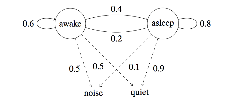
Note that when we are at this step, that is, the calculations for the Viterbi Algorithm to find the most likely tag sequence given a set of observations over a series of time steps, we assume that transition and emission probabilities have already been calculated from the given corpus. Let’s have a look at a sample of transition and emission probabilities for the baby sleeping problem that we would use for our calculations of the algorithm.
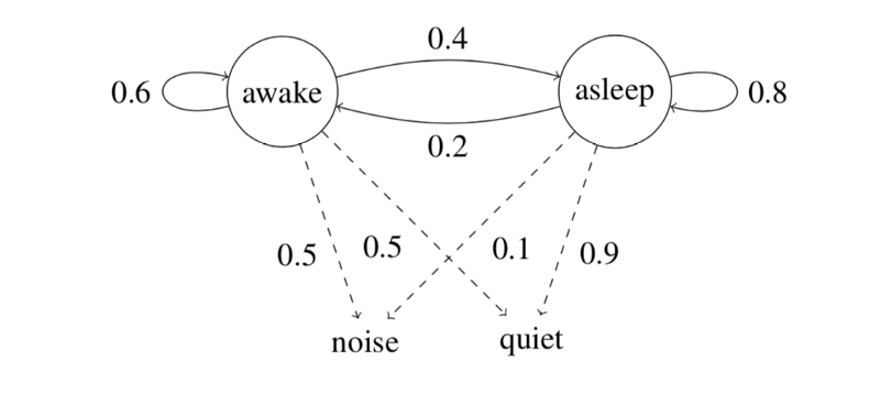
The baby starts by being awake, and remains in the room for three time points, t1 . . . t3 (three iterations of the Markov chain). The observations are: quiet, quiet, noise. Have a look at the following diagram that shows the calculations for up to two time-steps. The complete diagram with all the final set of values will be shown afterwards.
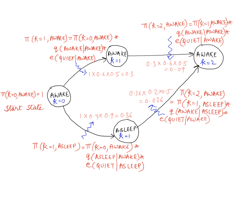
We have not shown the calculations for the state of “asleep” at k = 2 and the calculations for k = 3 in the above diagram to keep things simple.
Now that we have all these calculations in place, we want to calculate the most likely sequence of states that the baby can be in over the different given time steps. So, for k = 2 and the state of Awake, we want to know the most likely state at k = 1 that transitioned to Awake at k = 2. (k = 2 represents a sequence of states of length 3 starting off from 0 and t = 2 would mean the state at time-step 2. We are given the state at t = 0 i.e. Awake).
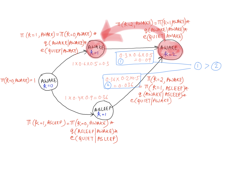
Clearly, if the state at time-step 2 was AWAKE, then the state at time-step 1 would have been AWAKE as well, as the calculations point out. So, the Viterbi Algorithm not only helps us find the π(k) values, that is the cost values for all the sequences using the concept of dynamic programming, but it also helps us to find the most likely tag sequence given a start state and a sequence of observations. The algorithm, along with the pseudo-code for storing the back-pointers is given below.
Calculations for the Part of Speech Tagging Problem
Let us look at a slightly bigger corpus for the part of speech tagging and the corresponding Viterbi graph showing the calculations and back-pointers for the Viterbi Algorithm.
Here is the corpus that we will consider:
Now take a look at the transition probabilities calculated from this corpus.
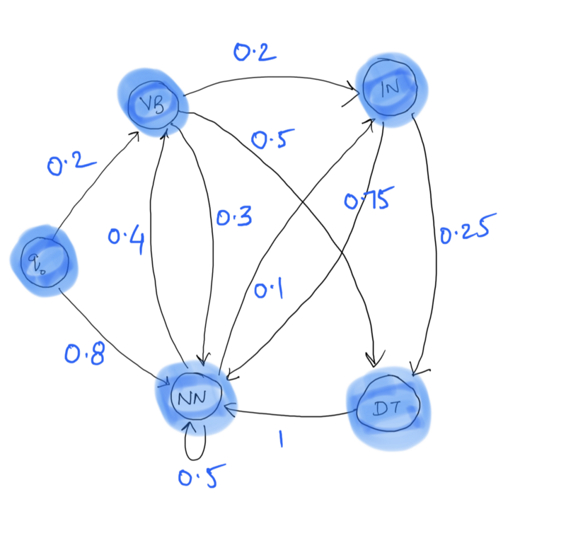
Here, q0 → VB represents the probability of a sentence starting off with the tag VB, that is the first word of a sentence being tagged as VB. Similarly, q0 → NN represents the probability of a sentence starting with the tag NN. Notice that out of 10 sentences in the corpus, 8 start with NN and 2 with VB and hence the corresponding transition probabilities.
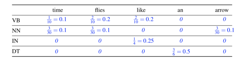
As for the emission probabilities, ideally we should be looking at all the combinations of tags and words in the corpus. Since that would be too much, we will only consider emission probabilities for the sentence that would be used in the calculations for the Viterbi Algorithm.
Time flies like an arrow
The emission probabilities for the sentence above are:
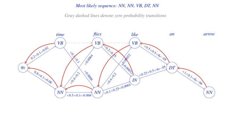
Finally, we are ready to see the calculations for the given sentence, transition probabilities, emission probabilities, and the given corpus.
So, is that all there is to the Viterbi Algorithm ?
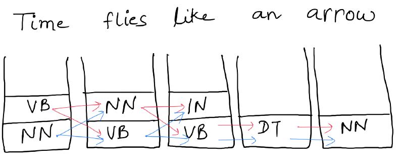
Take a look at the example below.
The bucket below each word is filled with the possible tags seen next to the word in the training corpus. The given sentence can have the combinations of tags depending on which path we take. But there is a catch. Can you figure out what that is?
Were you able to figure it out?
No??
Let me tell you what it is.
There might be some path in the computation graph for which we do not have a transition probability. So our algorithm can just discard that path and take the other path.
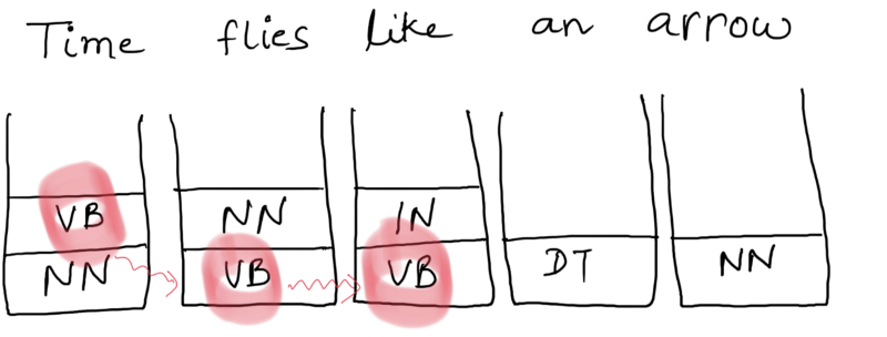
In the above diagram, we discard the path marked in red since we do not have q(VB|VB). The training corpus never has a VB followed by VB. So in the Viterbi calculations, we end up taking q(VB|VB) = 0. And if you’ve been following the algorithm along closely, you would find that a single 0 in the calculations would make the entire probability or the maximum cost for a sequence of tags / labels to be 0.
This however means that we are ignoring the combinations which are not seen in the training corpus.
Is that the right way to approach the real world examples?
Consider a small tweak in the above sentence.
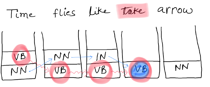
In this sentence we do not have any alternative path. Even if we have Viterbi probability until we reach the word “like”, we cannot proceed further. Since both q(VB|VB) = 0 and q(VB|IN) = 0. What do we do now?
The corpus that we considered here was very small. Consider any reasonably sized corpus with a lot of words and we have a major problem of sparsity of data. Take a look below.
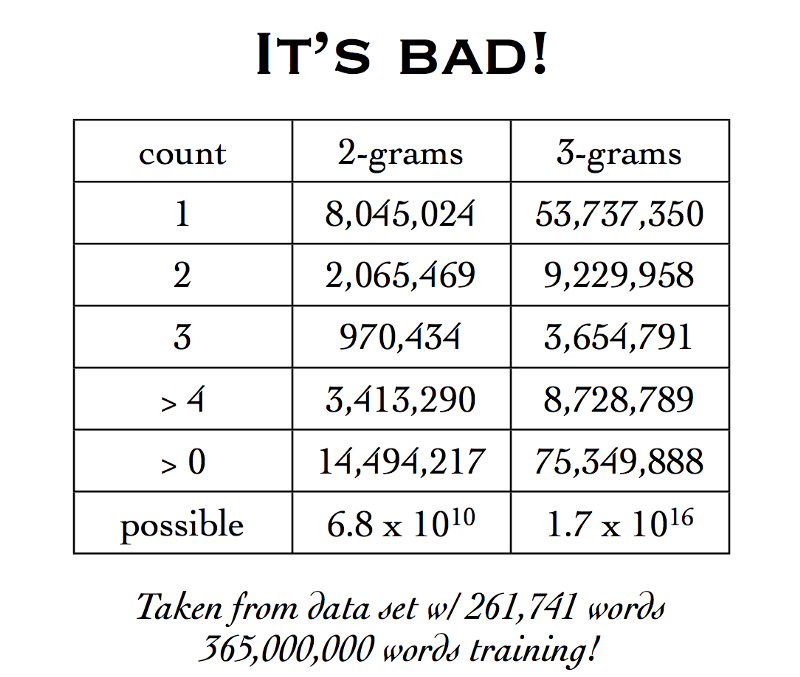
That means that we can have a potential 68 billion bigrams but the number of words in the corpus are just under a billion. That is a huge number of zero transition probabilities to fill up. The problem of sparsity of data is even more elaborate in case we are considering trigrams.
To solve this problem of data sparsity, we resort to a solution called Smoothing.
Smoothing
The idea behind Smoothing is just this:
- Discount — the existing probability values somewhat and
- Reallocate — this probability to the zeroes
In this way, we redistribute the non zero probability values to compensate for the unseen transition combinations. Let us consider a very simple type of smoothing technique known as Laplace Smoothing.
Laplace smoothing is also known as one count smoothing. You will understand exactly why it goes by that name in a moment. Let’s revise how the parameters for a trigram HMM model are calculated given a training corpus.
The possible values that can go wrong here are
c(u, v, s)is 0c(u, v)is 0- We get an unknown word in the test sentence, and we don’t have any training tags associated with it.
All these can be solved via smoothing. So the Laplace smoothing counts would become
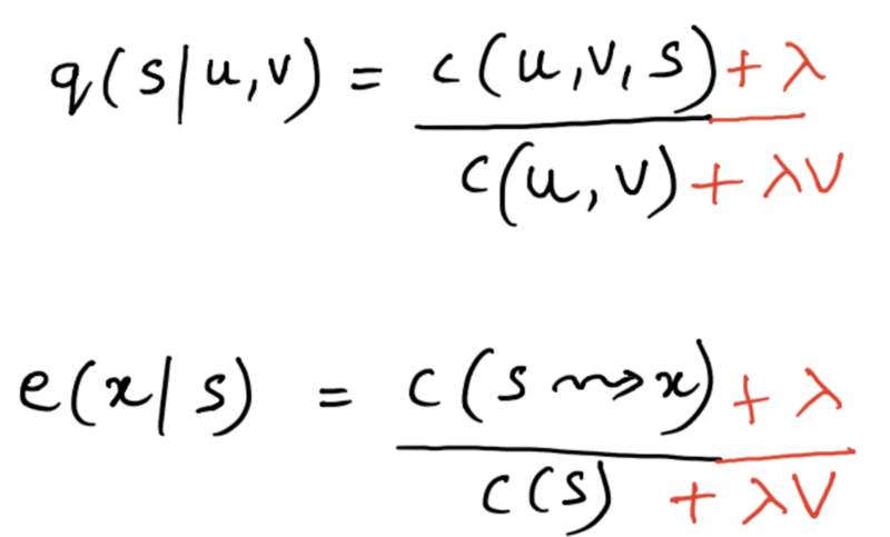
Here V is the total number of tags in our corpus and λ is basically a real value between 0 and 1. It acts like a discounting factor. A λ = 1 value would give us too much of a redistribution of values of probabilities. For example:
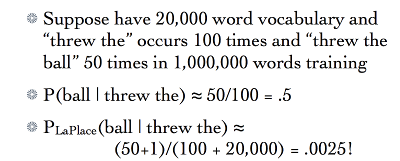
Too much of a weight is given to unseen trigrams for λ = 1 and that is why the above mentioned modified version of Laplace Smoothing is considered for all practical applications. The value of the discounting factor is to be varied from one application to another.
Note that λ = 1 would only create a problem if the vocabulary size is too large. For a smaller corpus, λ = 1 would give us a good performance to start off with.
A thing to note about Laplace Smoothing is that it is a uniform redistribution, that is, all the trigrams that were previously unseen would have equal probabilities. So, suppose we are given some data and we observe that
- Frequency of trigram is zero
- Frequency of trigram is also zero
- Uniform distribution over unseen events means:
P(thing|gave, the) = P(think|gave, the)
Does that reflect our knowledge about English use?
P(thing|gave, the) > P(think|gave, the) ideally, but uniform distribution using Laplace smoothing will not consider this.
This means that millions of unseen trigrams in a huge corpus would have equal probabilities when they are being considered in our calculations. That is probably not the right thing to do. However, it is better than to consider the 0 probabilities which would lead to these trigrams and eventually some paths in the Viterbi graph getting completely ignored. But this still needs to be worked upon and made better.
There are, however, a lot of different types of smoothing techniques that improve upon the basic Laplace Smoothing technique and help overcome this problem of uniform distribution of probabilities. Some of these techniques are:
- Good-Turing estimate
- Jelinek-Mercer smoothing (interpolation)
- Katz smoothing (backoff)
- Witten-Bell smoothing
- Absolute discounting
- Kneser-Ney smoothing
To read more on these different types of smoothing techniques in more detail, refer to this tutorial. Which smoothing technique to choose highly depends upon the type of application at hand, the type of data being considered, and also on the size of the data set.
If you have been following along this lengthy article, then I must say

Let’s move on and look at a slight optimization that we can do to the Viterbi algorithm that can reduce the number of computations and that also makes sense for a lot of data sets out there.
Before that, however, look at the pseudo-code for the algorithm once again.

If we look closely, we can see that for every trigram of words, we are considering all possible set of tags. That is, if the number of tags are V, then we are considering |V|³ number of combinations for every trigram of the test sentence.
Ignore the trigram for now and just consider a single word. We would be considering all of the unique tags for a given word in the above mentioned algorithm. Consider a corpus where we have the word “kick” which is associated with only two tags, say {NN, VB} and the total number of unique tags in the training corpus are around 500 (it’s a huge corpus).
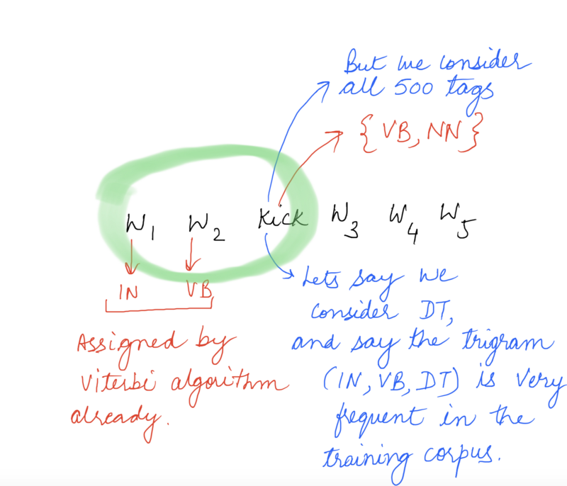
Now the problem here is apparent. We might end up assigning a tag that doesn’t make sense with the word under consideration, simply because the transition probability of the trigram ending at the tag was very high, like in the example shown above. Also, it would be computationally inefficient to consider all 500 tags for the word “kick” if it only ever occurs with two unique tags in the entire corpus.
So, the optimization we do is that for every word, instead of considering all the unique tags in the corpus, we just consider the tags that it occurred with in the corpus.
This would work because, for a reasonably large corpus, a given word would ideally occur with all the various set of tags with which it can occur (most of them at-least). Then it would be reasonable to simply consider just those tags for the Viterbi algorithm.
As far as the Viterbi decoding algorithm is concerned, the complexity still remains the same because we are always concerned with the worst case complexity. In the worst case, every word occurs with every unique tag in the corpus, and so the complexity remains at O(n|V|³) for the trigram model and O(n|V|²) for the bigram model.
For the recursive implementation of the code, please refer to
DivyaGodayal/HMM-POS-Tagger
_HMM-POS-Tagger — An HMM based Part of Speech Tagger implementation using Laplace Smoothing and Trigram HMMs_github.com
The recursive implementation is done along with Laplace Smoothing.
For the iterative implementation, refer to
edorado93/HMM-Part-of-Speech-Tagger
_HMM-Part-of-Speech-Tagger — An HMM based Part of Speech Tagger_github.com
This implementation is done with One-Count Smoothing technique which leads to better accuracy as compared to the Laplace Smoothing.
A lot of snapshots of formulas and calculations in the two articles are derived from [here](http://1. http://www.cs.columbia.edu/~mcollins/courses/nlp2011/notes/hmms.pdf).
Do let us know how this blog post helped you, and point out the mistakes if you find some while reading the article in the comments section below. Also, please recommend (by clapping) and spread the love as much as possible for this post if you think this might be useful for someone.