By Thomas Simonini
This article is part of Deep Reinforcement Learning Course with Tensorflow ?️. Check the syllabus here.
Last time, we learned about Q-Learning: an algorithm which produces a Q-table that an agent uses to find the best action to take given a state.
But as we’ll see, producing and updating a Q-table can become ineffective in big state space environments.
This article is the third part of a series of blog post about Deep Reinforcement Learning. For more information and more resources, check out the syllabus of the course.
Today, we’ll create a Deep Q Neural Network. Instead of using a Q-table, we’ll implement a Neural Network that takes a state and approximates Q-values for each action based on that state.
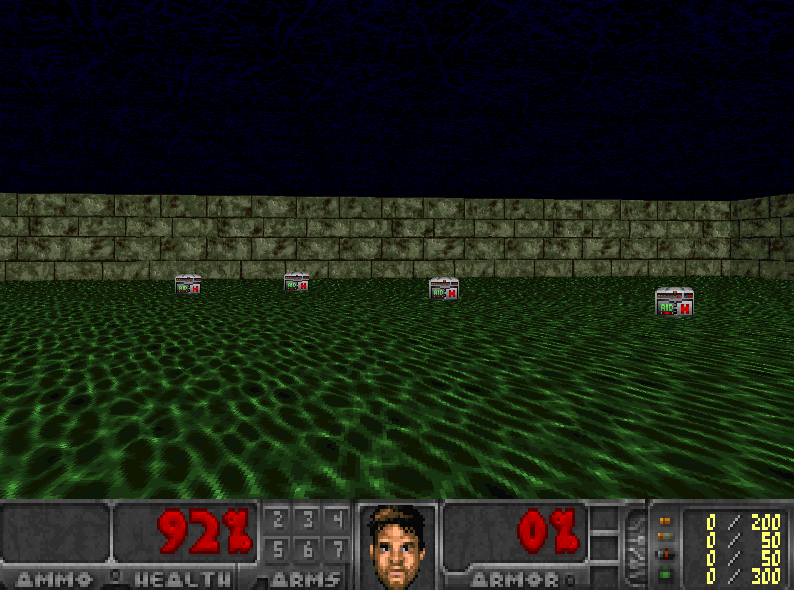
Thanks to this model, we’ll be able to create an agent that learns to play Doom!
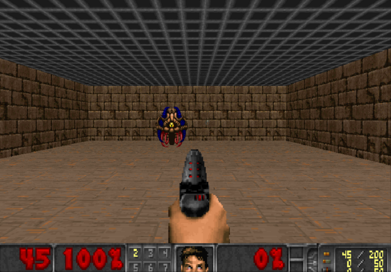
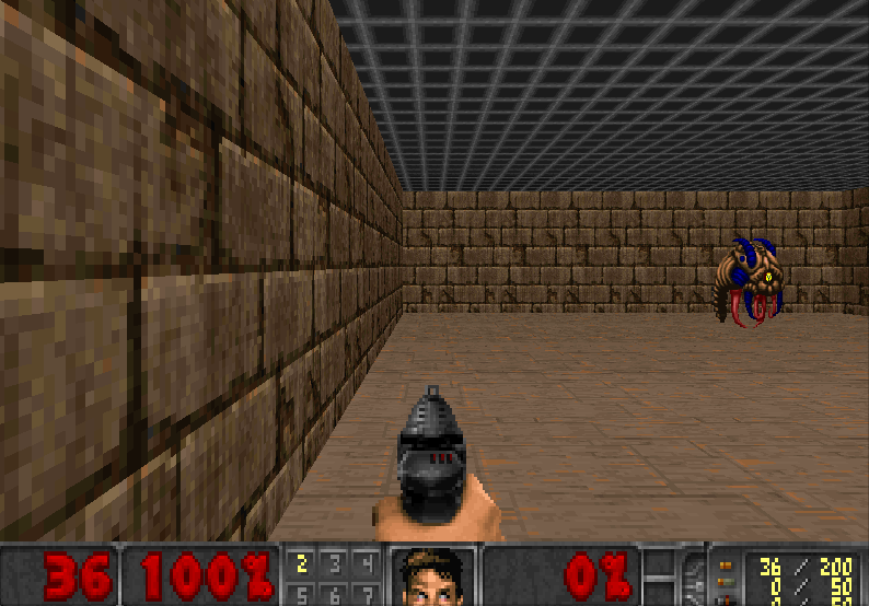 Our DQN Agent
In this article you’ll learn:
- What is Deep Q-Learning (DQL)?
- What are the best strategies to use with DQL?
- How to handle the temporal limitation problem
- Why we use experience replay
- What are the mathematics behind DQL
- How to implement it in Tensorflow
Adding ‘Deep’ to Q-Learning
In the last article, we created an agent that plays Frozen Lake thanks to the Q-learning algorithm.
We implemented the Q-learning function to create and update a Q-table. Think of this as a “cheat-sheet” to help us to find the maximum expected future reward of an action, given a current state. This was a good strategy — however, this is not scalable.
Imagine what we’re going to do today. We’ll create an agent that learns to play Doom. Doom is a big environment with a gigantic state space (millions of different states). Creating and updating a Q-table for that environment would not be efficient at all.
The best idea in this case is to create a neural network that will approximate, given a state, the different Q-values for each action.
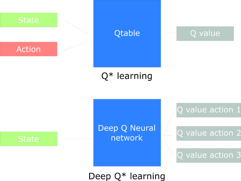
How does Deep Q-Learning work?
This will be the architecture of our Deep Q Learning:
This can seem complex, but I’ll explain the architecture step by step.
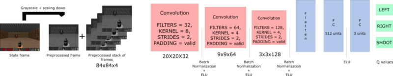
Our Deep Q Neural Network takes a stack of four frames as an input. These pass through its network, and output a vector of Q-values for each action possible in the given state. We need to take the biggest Q-value of this vector to find our best action.
In the beginning, the agent does really badly. But over time, it begins to associate frames (states) with best actions to do.
Preprocessing part
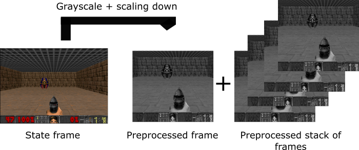
Preprocessing is an important step. We want to reduce the complexity of our states to reduce the computation time needed for training.
First, we can grayscale each of our states. Color does not add important information (in our case, we just need to find the enemy and kill him, and we don’t need color to find him). This is an important saving, since we reduce our three colors channels (RGB) to 1 (grayscale).
Then, we crop the frame. In our example, seeing the roof is not really useful.
Then we reduce the size of the frame, and we we stack four sub-frames together.
The problem of temporal limitation
Arthur Juliani gives an awesome explanation about this topic in his article. He has a clever idea: using LSTM neural networks for handling the problem.
However, I think it’s better for beginners to use stacked frames.
The first question that you can ask is why we stack frames together?
We stack frames together because it helps us to handle the problem of temporal limitation.
Let’s take an example, in the game of Pong. When you see this frame:

Can you tell me where the ball is going?
No, because one frame is not enough to have a sense of motion!
But what if I add three more frames? Here you can see that the ball is going to the right.

That’s the same thing for our Doom agent. If we give him only one frame at a time, it has no idea of motion. And how can it make a correct decision, if it can’t determine where and how fast objects are moving?
Using convolution networks
The frames are processed by three convolution layers. These layers allow you to exploit spatial relationships in images. But also, because frames are stacked together, you can exploit some spatial properties across those frames.
If you’re not familiar with convolution, please read this excellent intuitive article by Adam Geitgey.
Each convolution layer will use ELU as an activation function. ELU has been proven to be a good activation function for convolution layers.
We use one fully connected layer with ELU activation function and one output layer (a fully connected layer with a linear activation function) that produces the Q-value estimation for each action.
Experience Replay: making more efficient use of observed experience
Experience replay will help us to handle two things:
- Avoid forgetting previous experiences.
- Reduce correlations between experiences.
I will explain these two concepts.
This part and the illustrations were inspired by the great explanation in the Deep Q Learning chapter in the Deep Learning Foundations Nanodegree by Udacity.
Avoid forgetting previous experiences
We have a big problem: the variability of the weights, because there is high correlation between actions and states.
Remember in the first article (Introduction to Reinforcement Learning), we spoke about the Reinforcement Learning process:
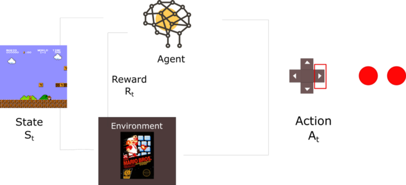
At each time step, we receive a tuple (state, action, reward, new_state). We learn from it (we feed the tuple in our neural network), and then throw this experience.
Our problem is that we give sequential samples from interactions with the environment to our neural network. And it tends to forget the previous experiences as it overwrites with new experiences.
For instance, if we are in the first level and then the second (which is totally different), our agent can forget how to behave in the first level.
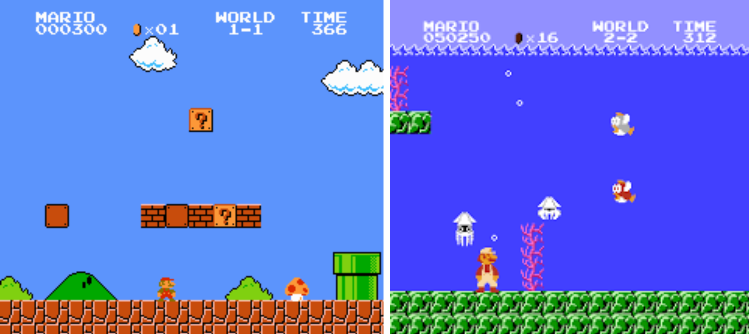 By learning how to play on water level, our agent will forget how to behave on the first level
As a consequence, it can be more efficient to make use of previous experience, by learning with it multiple times.
Our solution: create a “replay buffer.” This stores experience tuples while interacting with the environment, and then we sample a small batch of tuple to feed our neural network.
Think of the replay buffer as a folder where every sheet is an experience tuple. You feed it by interacting with the environment. And then you take some random sheet to feed the neural network
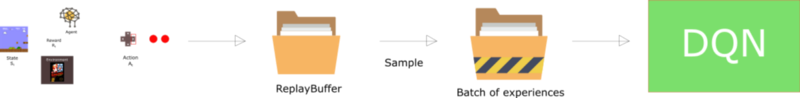
This prevents the network from only learning about what it has immediately done.
Reducing correlation between experiences
We have another problem — we know that every action affects the next state. This outputs a sequence of experience tuples which can be highly correlated.
If we train the network in sequential order, we risk our agent being influenced by the effect of this correlation.
By sampling from the replay buffer at random, we can break this correlation. This prevents action values from oscillating or diverging catastrophically.
It will be easier to understand that with an example. Let’s say we play a first-person shooter, where a monster can appear on the left or on the right. The goal of our agent is to shoot the monster. It has two guns and two actions: shoot left or shoot right.
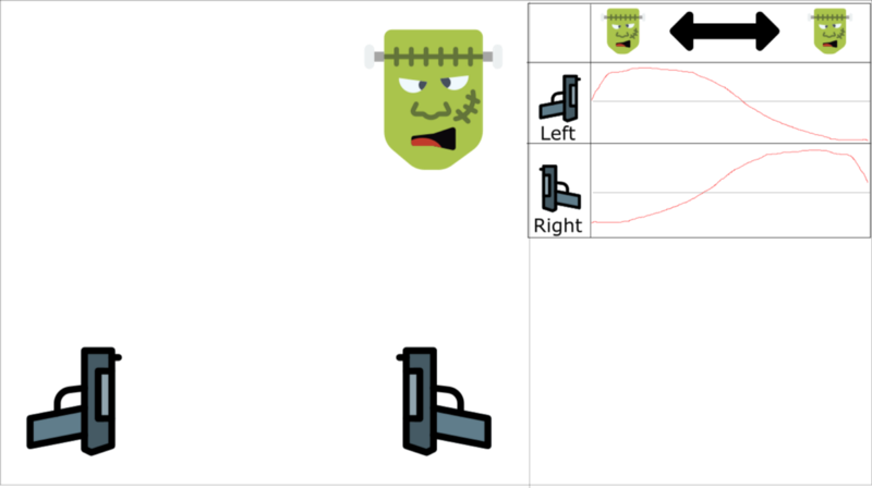 The table represents the Q-values approximations
We learn with ordered experience. Say we know that if we shoot a monster, the probability that the next monster comes from the same direction is 70%. In our case, this is the correlation between our experiences tuples.
Let’s begin the training. Our agent sees the monster on the right, and shoots it using the right gun. This is correct!
Then the next monster also comes from the right (with 70% probability), and the agent will shoot with the right gun. Again, this is good!
And so on and on…
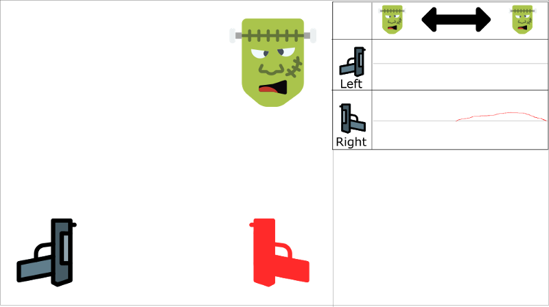 Red gun is the action taken
The problem is, this approach increases the value of using the right gun through the entire state space.
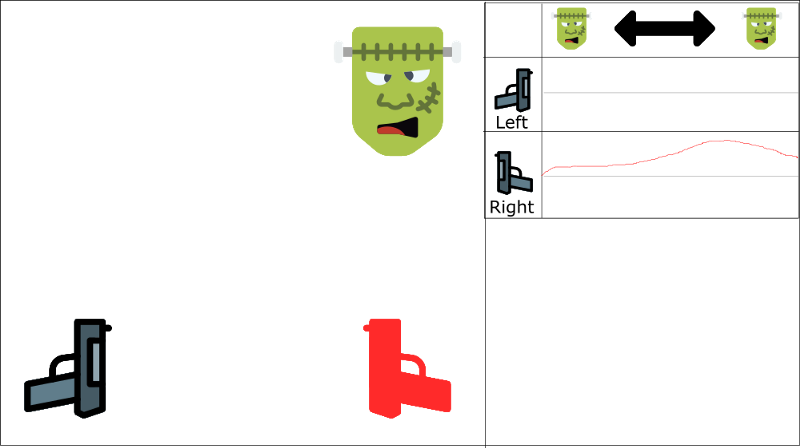 We can see that the Q-value for monster being at left and shooting with right gun is positive (even if it’s not rational)
And if our agent doesn’t see a lot of left examples (since only 30% will probably come from the left), our agent will only finish by choosing right regardless of where the monster comes from. This is not rational at all.
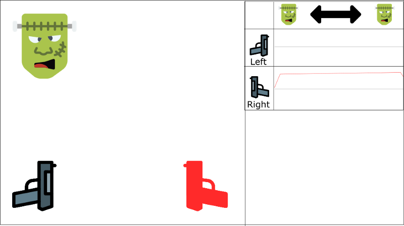 Even if the monster comes to the left, our agent will shoot with the right gun
We have two parallel strategies to handle this problem.
First, we must stop learning while interacting with the environment. We should try different things and play a little randomly to explore the state space. We can save these experiences in the replay buffer.
Then, we can recall these experiences and learn from them. After that, go back to play with updated value function.
As a consequence, we will have a better set of examples. We will be able to generalize patterns from across these examples, recalling them in whatever order.
This helps avoid being fixated on one region of the state space. This prevents reinforcing the same action over and over.
This approach can be seen as a form of Supervised Learning.
We’ll see in future articles that we can also use “prioritized experience replay.” This lets us present rare or “important” tuples to the neural network more frequently.
Our Deep Q-Learning algorithm
First a little bit of mathematics:
Remember that we update our Q value for a given state and action using the Bellman equation:
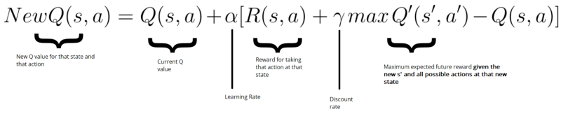
In our case, we want to update our neural nets weights to reduce the error.
The error (or TD error) is calculated by taking the difference between our Q_target (maximum possible value from the next state) and Q_value (our current prediction of the Q-value)
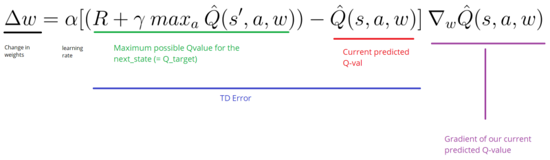
Initialize Doom Environment EInitialize replay Memory M with capacity N (= finite capacity)Initialize the DQN weights wfor episode in max_episode: s = Environment state for steps in max_steps: Choose action a from state s using epsilon greedy. Take action a, get r (reward) and s' (next state) Store experience tuple <s, a, r, s'> in M s = s' (state = new_state) Get random minibatch of exp tuples from M Set Q_target = reward(s,a) + γmaxQ(s') Update w = α(Q_target - Q_value) * ∇w Q_value
There are two processes that are happening in this algorithm:
- We sample the environment where we perform actions and store the observed experiences tuples in a replay memory.
- Select the small batch of tuple random and learn from it using a gradient descent update step.
Let’s implement our Deep Q Neural Network
We made a video where we implement a Deep Q-learning agent with Tensorflow that learns to play Atari Space Invaders ?️?.
Now that we know how it works, we’ll implement our Deep Q Neural Network step by step. Each step and each part of the code is explained directly in the Jupyter notebook linked below.
You can access it in the Deep Reinforcement Learning Course repo.
That’s all! You’ve just created an agent that learns to play Doom. Awesome!
Don’t forget to implement each part of the code by yourself. It’s really important to try to modify the code I gave you. Try to add epochs, change the architecture, add fixed Q-values, change the learning rate, use a harder environment (such as Health Gathering)…and so on.Have fun!
In the next article, I will discuss the last improvements in Deep Q-learning:
- Fixed Q-values
- Prioritized Experience Replay
- Double DQN
- Dueling Networks
But next time we’ll work on Policy Gradients by training an agent that plays Doom, and we’ll try to survive in an hostile environment by collecting health.
If you liked my article, please click the ? below as many time as you liked the article so other people will see this here on Medium. And don’t forget to follow me!
If you have any thoughts, comments, questions, feel free to comment below or send me an email: hello@simoninithomas.com, or tweet me @ThomasSimonini.


Keep learning, stay awesome!
Deep Reinforcement Learning Course with Tensorflow ?️
? Syllabus
? Video version
Part 1: An introduction to Reinforcement Learning
Part 2: Diving deeper into Reinforcement Learning with Q-Learning
Part 3: An introduction to Deep Q-Learning: let’s play Doom
Part 4: An introduction to Policy Gradients with Doom and Cartpole
Part 5: An intro to Advantage Actor Critic methods: let’s play Sonic the Hedgehog!
Part 6: Proximal Policy Optimization (PPO) with Sonic the Hedgehog 2 and 3