By Déborah Mesquita
Developers often say that if you want to get started with machine learning, you should first learn how the algorithms work. But my experience shows otherwise.
I say you should first be able to see the big picture: how the applications work. Once you understand this, it becomes much easier to dive in deep and explore the inner workings of the algorithms.
So how do you develop an intuition and achieve this big-picture understanding of machine learning? A good way to do this is by creating machine learning models.
Assuming you still don’t know how to create all these algorithms from scratch, you’ll want to use a library that has all these algorithms already implemented for you. And that library is TensorFlow.
In this article, we’ll create a machine learning model to classify texts into categories. We’ll cover the following topics:
- How TensorFlow works
- What is a machine learning model
- What is a Neural Network
- How the Neural Network learns
- How to manipulate data and pass it to the Neural Network inputs
- How to run the model and get the prediction results
You will probably learn a lot of new things, so let’s start! ?
TensorFlow
TensorFlow is an open-source library for machine learning, first created by Google. The name of the library help us understand how we work with it: tensors are multidimensional arrays that flow through the nodes of a graph.
tf.Graph
Every computation in TensorFlow is represented as a dataflow graph. This graph has two elements:
- a set of
tf.Operation, that represents units of computation - a set of
tf.Tensor, that represents units of data
To see how all this works you will create this dataflow graph:

You’ll define x = [1,3,6] and y = [1,1,1]. As the graph works with tf.Tensor to represent units of data, you will create constant tensors:
import tensorflow as tf
x = tf.constant([1,3,6]) y = tf.constant([1,1,1])
Now you’ll define the operation unit:
import tensorflow as tf
x = tf.constant([1,3,6]) y = tf.constant([1,1,1])
op = tf.add(x,y)
You have all the graph elements. Now you need to build the graph:
import tensorflow as tf
my_graph = tf.Graph()
with my_graph.as_default(): x = tf.constant([1,3,6]) y = tf.constant([1,1,1])
op = tf.add(x,y)
This is how the TensorFlow workflow works: you first create a graph, and only then can you make the computations (really ‘running’ the graph nodes with operations). To run the graph you’ll need to create a tf.Session.
tf.Session
A tf.Session object encapsulates the environment in which Operation objects are executed, and Tensor objects are evaluated (from the docs). To do that, we need to define which graph will be used in the Session:
import tensorflow as tf
my_graph = tf.Graph()
with tf.Session(graph=my_graph) as sess: x = tf.constant([1,3,6]) y = tf.constant([1,1,1])
op = tf.add(x,y)
To execute the operations, you’ll use the method tf.Session.run(). This method executes one ‘step’ of the TensorFlow computation, by running the necessary graph fragment to execute every Operation objects and evaluate every Tensor passed in the argument fetches. In your case you will run a step of the sum operations:
import tensorflow as tf
my_graph = tf.Graph()
with tf.Session(graph=my_graph) as sess: x = tf.constant([1,3,6]) y = tf.constant([1,1,1])
op = tf.add(x,y) result = sess.run(fetches=op) print(result)
>>>; [2 4 7]
A Predictive Model
Now that you know how TensorFlow works, you have to learn how to create a predictive model. In short,
Machine learning algorithm + data = predictive model
The process to construct a model is like this:
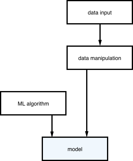
As you can see, the model consists of a machine learning algorithm ‘trained’ with data. When you have the model you will get results like this:

The goal of the model you will create is to classify texts in categories, we define that:
input: text, result: category
We have a training dataset with all the texts labeled (every text has a label indicating to which category it belongs). In machine learning this type of task is denominated Supervised learning.
“We know the correct answers. The algorithm iteratively makes predictions on the training data and is corrected by the teacher.” — Jason Brownlee
You’ll classify data into categories, so it’s also a Classification task.
To create the model, we’re going to use Neural Networks.
Neural Networks
A neural network is a computational model (a way to describe a system using mathematical language and mathematical concepts). These systems are self-learning and trained, rather than explicitly programmed.
Neural networks are inspired by our central nervous system. They have connected nodes that are similar to our neurons.
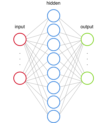
The Perceptron was the first neural network algorithm. This article explains really well the inner working of a perceptron (the “Inside an artificial neuron” animation is fantastic).
To understand how a neural network works we will actually build a neural network architecture with TensorFlow. This architecture was used by Aymeric Damien in this example.
Neural Network architecture
The neural network will have 2 hidden layers (you have to choose how many hidden layers the network will have, is part of the architecture design). The job of each hidden layer is to transform the inputs into something that the output layer can use.
Hidden layer 1
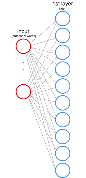
You also need to define how many nodes the 1st hidden layer will have. These nodes are also called features or neurons, and in the image above they are represented by each circle.
In the input layer every node corresponds to a word of the dataset (we will see how this works later).
As explained here, each node (neuron) is multiplied by a weight. Every node has a weight value, and during the training phase the neural network adjusts these values in order to produce a correct output (wait, we will learn more about this in a minute).
In addition to multiplying each input node by a weight, the network also adds a bias (role of bias in neural networks).
In your architecture after multiplying the inputs by the weights and sum the values to the bias, the data also pass by an activation function. This activation function defines the final output of each node. An analogy: imagine that each node is a lamp, the activation function tells if the lamp will light or not.
There are many types of activation functions. You will use the rectified linear unit (ReLu). This function is defined this way:
f(x) = max(0,x) [the output is x or 0 (zero), whichever is larger]
Examples: ifx = -1, then f(x) = 0(zero); if x = 0.7, then f(x) = 0.7.
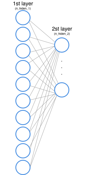
Hidden layer 2
The 2nd hidden layer does exactly what the 1st hidden layer does, but now the input of the 2nd hidden layer is the output of the 1st one.
Output layer
And we finally got to the last layer, the output layer. You will use the one-hot encoding to get the results of this layer. In this encoding only one bit has the value 1 and all the other ones got a zero value. For example, if we want to encode three categories (sports, space and computer graphics):
+-------------------+-----------+| category | value |+-------------------|-----------+| sports | 001 || space | 010 || computer graphics | 100 ||-------------------|-----------|
So the number of output nodes is the number of classes of the input dataset.
The output layer values are also multiplied by the weights and we also add the bias, but now the activation function is different.
You want to label each text with a category, and these categories are mutually exclusive (a text doesn’t belong to two categories at the same time). To consider this, instead of using the ReLu activation function you will use the Softmax function. This function transforms the output of each unity to a value between 0 and 1 and also makes sure that the sum of all units equals 1. This way the output will tell us the probability of each text for each category.
| 1.2 0.46|| 0.9 -> [softmax] -> 0.34|| 0.4 0.20|
And now you have the data flow graph of your neural network. Translating everything we saw so far into code, the result is:
# Network Parametersn_hidden_1 = 10 # 1st layer number of featuresn_hidden_2 = 5 # 2nd layer number of featuresn_input = total_words # Words in vocabn_classes = 3 # Categories: graphics, space and baseball
def multilayer_perceptron(input_tensor, weights, biases): layer_1_multiplication = tf.matmul(input_tensor, weights['h1']) layer_1_addition = tf.add(layer_1_multiplication, biases['b1']) layer_1_activation = tf.nn.relu(layer_1_addition)
# Hidden layer with RELU activation layer_2_multiplication = tf.matmul(layer_1_activation, weights['h2']) layer_2_addition = tf.add(layer_2_multiplication, biases['b2']) layer_2_activation = tf.nn.relu(layer_2_addition)
# Output layer with linear activation out_layer_multiplication = tf.matmul(layer_2_activation, weights['out']) out_layer_addition = out_layer_multiplication + biases['out']
return out_layer_addition
(We’ll talk about the code for the output layer activation function later.)
How the neural network learns
As we saw earlier the weight values are updated while the network is trained. Now we will see how this happens in the TensorFlow environment.
tf.Variable
The weights and biases are stored in variables (tf.Variable). These variables maintain state in the graph across calls to run(). In machine learning we usually start the weight and bias values through a normal distribution.
weights = { 'h1': tf.Variable(tf.random_normal([n_input, n_hidden_1])), 'h2': tf.Variable(tf.random_normal([n_hidden_1, n_hidden_2])), 'out': tf.Variable(tf.random_normal([n_hidden_2, n_classes]))}biases = { 'b1': tf.Variable(tf.random_normal([n_hidden_1])), 'b2': tf.Variable(tf.random_normal([n_hidden_2])), 'out': tf.Variable(tf.random_normal([n_classes]))}
When we run the network for the first time (that is, the weight values are the ones defined by the normal distribution):
input values: xweights: wbias: boutput values: z
expected values: expected
To know if the network is learning or not, you need to compare the output values (z) with the expected values (expected). And how do we compute this difference (loss)? There are many methods to do that. Because we are working with a classification task, the best measure for the loss is the cross-entropy error.
James D. McCaffrey wrote a brilliant explanation about why this is the best method for this kind of task.
With TensorFlow you will compute the cross-entropy error using the tf.nn.softmax_cross_entropy_with_logits() method (here is the softmax activation function) and calculate the mean error (tf.reduce_mean()).
# Construct modelprediction = multilayer_perceptron(input_tensor, weights, biases)
# Define lossentropy_loss = tf.nn.softmax_cross_entropy_with_logits(logits=prediction, labels=output_tensor)loss = tf.reduce_mean(entropy_loss)
You want to find the best values for the weights and biases in order to minimize the output error (the difference between the value we got and the correct value). To do that you will use the gradient descent method. To be more specific, you will use the stochastic gradient descent.
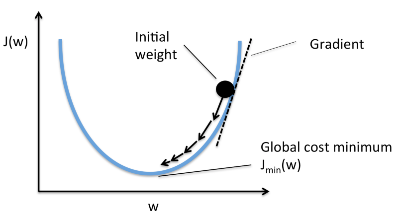
There are also many algorithms to compute the gradient descent, you will use the Adaptive Moment Estimation (Adam). To use this algorithm in TensorFlow you need to pass the learning_rate value, that determines the incremental steps of the values to find the best weight values.
The method tf.train.AdamOptimizer(learning_rate)**.minimize(loss)** is a syntactic sugar that does two things:
- compute_gradients(loss, )
- apply_gradients()
The method updates all the tf.Variables with the new values, so we don’t need to pass the list of variables. And now you have the code to train the network:
learning_rate = 0.001
# Construct modelprediction = multilayer_perceptron(input_tensor, weights, biases)
# Define lossentropy_loss = tf.nn.softmax_cross_entropy_with_logits(logits=prediction, labels=output_tensor)loss = tf.reduce_mean(entropy_loss)
optimizer = tf.train.AdamOptimizer(learning_rate=learning_rate).minimize(loss)
Data manipulation
The dataset you will use has many texts in English and we need to manipulate this data to pass it to the neural network. To do that you will do two things:
- Create an index for each word
- Create a matrix for each text, where the values are 1 if a word is in the text and 0 if not
Let’s see the code to understand this process:
import numpy as np #numpy is a package for scientific computingfrom collections import Counter
vocab = Counter()
text = "Hi from Brazil"
#Get all wordsfor word in text.split(' '): vocab[word]+=1 #Convert words to indexesdef get_word_2_index(vocab): word2index = {} for i,word in enumerate(vocab): word2index[word] = i return word2index
#Now we have an indexword2index = get_word_2_index(vocab)
total_words = len(vocab)
#This is how we create a numpy array (our matrix)matrix = np.zeros((total_words),dtype=float)
#Now we fill the valuesfor word in text.split(): matrix[word2index[word]] += 1
print(matrix)
>>> [ 1. 1. 1.]
In the example above the text was ‘Hi from Brazil’ and the matrix was [ 1. 1. 1.]. What if the text was only ‘Hi’?
matrix = np.zeros((total_words),dtype=float)
text = "Hi"
for word in text.split(): matrix[word2index[word.lower()]] += 1
print(matrix)
>>> [ 1. 0. 0.]
You will to the same with the labels (categories of the texts), but now you will use the one-hot encoding:
y = np.zeros((3),dtype=float)
if category == 0: y[0] = 1. # [ 1. 0. 0.]elif category == 1: y[1] = 1. # [ 0. 1. 0.]else: y[2] = 1. # [ 0. 0. 1.]
Running the graph and getting the results
Now comes the best part: getting the results from the model. First let’s take a closer look at the input dataset.
The dataset
You will use the 20 Newsgroups, a dataset with 18.000 posts about 20 topics. To load this dataset you will use the scikit-learn library. We will use only 3 categories: comp.graphics, sci.space and rec.sport.baseball. The scikit-learn has two subsets: one for training and one for testing. The recommendation is that you should never look at the test data, because this can interfere in your choices while creating the model. You don’t want to create a model to predict this specific test data, you want to create a model with a good generalization.
This is how you will load the datasets:
from sklearn.datasets import fetch_20newsgroups
categories = ["comp.graphics","sci.space","rec.sport.baseball"]
newsgroups_train = fetch_20newsgroups(subset='train', categories=categories)newsgroups_test = fetch_20newsgroups(subset='test', categories=categories)
Training the model
In the neural network terminology, one epoch = one forward pass (getting the output values) and one backward pass (updating the weights) of all the training examples.
Remember the tf.Session.run() method? Let’s take a closer look at it:
tf.Session.run(fetches, feed_dict=None, options=None, run_metadata=None)
In the dataflow graph of the beginning of this article you used the sum operation, but we can also pass a list of things to run. In this neural network run you will pass two things: the loss calculation and the optimization step.
The feed_dict parameter is where we pass the data for each run step. To pass this data we need to define tf.placeholders (to feed the feed_dict).
As the TensorFlow documentation says:
“A placeholder exists solely to serve as the target of feeds. It is not initialized and contains no data.” — Source
So you will define your placeholders like this:
n_input = total_words # Words in vocabn_classes = 3 # Categories: graphics, sci.space and baseball
input_tensor = tf.placeholder(tf.float32,[None, n_input],name="input")output_tensor = tf.placeholder(tf.float32,[None, n_classes],name="output")
You will separate the training data in batches:
“If you use placeholders for feeding input, you can specify a variable batch dimension by creating the placeholder with tf.placeholder(…, shape=[None, …]). The None element of the shape corresponds to a variable-sized dimension.” — Source
We will feed the dict with a larger batch while testing the model, that’s why you need to the define a variable batch dimension.
The get_batches() function gives us the number of texts with the size of the batch. And now we can run the model:
training_epochs = 10
# Launch the graphwith tf.Session() as sess: sess.run(init) #inits the variables (normal distribution, remember?)
# Training cycle for epoch in range(training_epochs): avg_cost = 0. total_batch = int(len(newsgroups_train.data)/batch_size) # Loop over all batches for i in range(total_batch): batch_x,batch_y = get_batch(newsgroups_train,i,batch_size) # Run optimization op (backprop) and cost op (to get loss value) c,_ = sess.run([loss,optimizer], feed_dict={input_tensor: batch_x, output_tensor:batch_y})
Now you have the model, trained. To test it, you’ll also need to create graph elements. We’ll measure the accuracy of the model, so you need to get the index of the predicted value and the index of the correct value (because we are using the one-hot encoding), check is they are equal and calculate the mean to all the test dataset:
# Test model index_prediction = tf.argmax(prediction, 1) index_correct = tf.argmax(output_tensor, 1) correct_prediction = tf.equal(index_prediction, index_correct)
# Calculate accuracy accuracy = tf.reduce_mean(tf.cast(correct_prediction, "float")) total_test_data = len(newsgroups_test.target) batch_x_test,batch_y_test = get_batch(newsgroups_test,0,total_test_data) print("Accuracy:", accuracy.eval({input_tensor: batch_x_test, output_tensor: batch_y_test}))
>>> Epoch: 0001 loss= 1133.908114347 Epoch: 0002 loss= 329.093700409 Epoch: 0003 loss= 111.876660109 Epoch: 0004 loss= 72.552971845 Epoch: 0005 loss= 16.673050320 Epoch: 0006 loss= 16.481995190 Epoch: 0007 loss= 4.848220565 Epoch: 0008 loss= 0.759822878 Epoch: 0009 loss= 0.000000000 Epoch: 0010 loss= 0.079848485 Optimization Finished!
Accuracy: 0.75
And that’s it! You created a model using a neural network to classify texts into categories. Congratulations! ?
You can see the notebook with the final code here.
Tip: modify the values we defined to see how the changes affect the training time and the model accuracy.
Any questions or suggestions? Leave them in the comments. Oh, and thank’s for reading! ? ✌?
Did you found this article helpful? I try my best to write a deep dive article each month, you can receive an email when I publish a new one.
It would mean a lot if you click the ? and share with friends. Follow me for more articles about Data Science and Machine Learning.
