By Bert Carremans
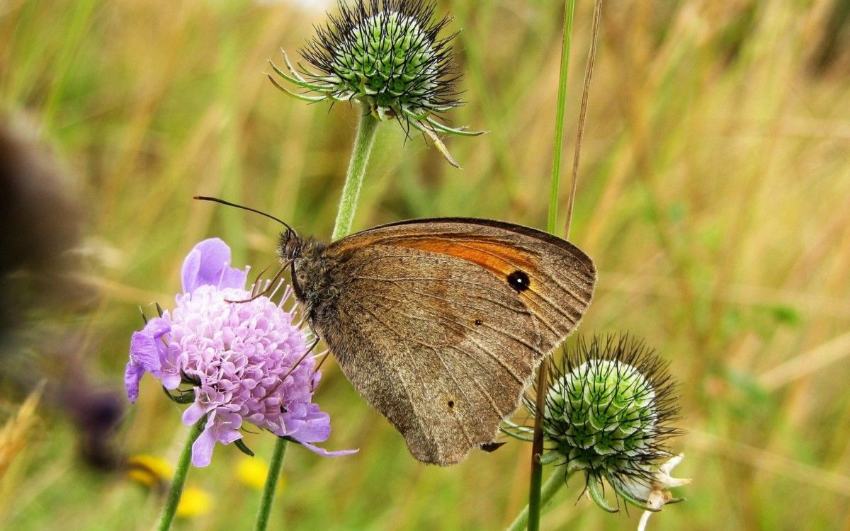
A while ago I read an interesting blog post on the website of the Dutch organization Vlinderstichting. Every year they organize a count of butterflies. Volunteers help in determining the different butterfly species in their garden. The Vlinderstichting gathers and analyses the results.
As the determination of the butterfly species is done by the volunteers, inevitably this process is prone to errors. As a result, the Vlinderstichting has to manually check the submissions, which is time-consuming.
Specifically, there are three butterflies for which the Vlinderstichting receives many wrong determinations. These are
- Meadow brown or Maniola jurtina
- Gatekeeper or Pyronia tithonus
- Small heath or Coenonympha pamphilus
In this article, I will describe the steps to fit a deep learning model that helps to make the distinction between the first two butterflies.
Downloading images with the Flickr API
To train a convolutional neural network I need to find images of butterflies with the correct label. Surely I could take pictures myself of the butterflies that I want to classify. They sometimes fly around in my garden…
Just kidding, that would take ages. For this, I need an automated way to get the images. To do that I use the Flickr API via Python.
Setting up the Flickr API
Firstly, I install the flickrapi package with pip. Then I create the necessary API keys on the Flickr website to connect to the Flickr API.
Besides the flickrapi package, I import the os and urllib packages for downloading the images and setting up the directories.
from flickrapi import FlickrAPI
import urllib
import os
import config
In the config module, I define the public and secret keys for the Flickr API. So this is simply a Python script (config.py) with the code below:
API_KEY = 'XXXXXXXXXXXXXXXXX'  // replace with your key
API_SECRET = 'XXXXXXXXXXXXXXXXX'  // replace with your secret
IMG_FOLDER = 'XXXXXXXXXXXXXXXXX'  // replace with your folder to store the images
I keep these keys in a separate file for security reasons. As a result, you can save the code in a public repository like GitHub or BitBucket and putting the config.py in .gitignore. Consequently, you can share your code with others while not having to worry about someone having access to your credentials.
To extract images of different butterfly species, I wrote a function download_flickr_photos. I will explain this function step by step. In addition, I’ve made the full code available on GitHub.
Input parameters
First of all, I check if the input parameters are of the correct type or values. If not, I raise an error. The explanation of the parameters can be found in the docstring of the function.
if not (isinstance(keywords, str) or isinstance(keywords, list)):
    raise AttributeError('keywords must be a string or a list of strings')
if not (size in ['thumbnail', 'square', 'medium', 'original']):
    raise AttributeError('size must be "thumbnail", "square", "medium" or "original"')
if not (max_nb_img == -1 or (max_nb_img > 0 and isinstance(max_nb_img, int))):
    raise AttributeError('max_nb_img must be an integer greater than zero or equal to -1')
Secondly, I define some of the parameters that will be used in the walk method later on. I create a list for the keywords and determine from which URL the images need to be downloaded.
if isinstance(keywords, str):
    keywords_list = []
    keywords_list.append(keywords)
else:
    keywords_list = keywords
if size == 'thumbnail':
    size_url = 'url_t'
elif size == 'square':
    size_url = 'url_q'
elif size == 'medium':
    size_url = 'url_c'
elif size == 'original':
    size_url = 'url_o'
Connecting to the Flickr API
Next, I connect to the Flickr API. In the FlickrAPI call I use the API keys defined in the config module.
flickr = FlickrAPI(config.API_KEY, config.API_SECRET)
Creating subfolders per butterfly species
I save the images of each butterfly species in a separate subfolder. The name of each subfolder is the butterfly species’ name, given by the keyword. If the subfolder does not exist yet, I create it.
results_folder = config.IMG_FOLDER + keyword.replace(" ", "_") + "/"
if not os.path.exists(results_folder):
    os.makedirs(results_folder)
Walking around in the Flickr library
photos = flickr.walk(
    text=keyword,
    extras='url_m',
    license='1,2,4,5',
    per_page=50)
I use the walk method of the Flickr API to search for images for the specified keyword. This walk method has the same parameters as the search method in the Flickr API.
In the text parameter, I use the keyword to search for images related to this keyword. Secondly, in the extras parameter, I specify url_m for a small, medium size of the images. More explanation on the image sizes and their respective URL is given in this Flickcurl C library.
Thirdly, in the license parameter, I select images with a non-commercial license. More on the license codes and their meaning can be found on the Flickr API platform. Finally, the per_page parameter specifies how many images I allow per page.
As a result, I have a generator called photos to download the images.
Downloading Flickr images
With the photos generator, I can download all the images found for the search query. First I get the specific URL at which I will download the image. Then I increment the count variable and use this counter to create the image filenames.
With the urlretrieve method, I download the image and save it in the folder for the butterfly species. If an error occurs I print out the error message.
for photo in photos:
    try:
        url=photo.get('url_m')
        print(url)
        count += 1
        urllib.request.urlretrieve(url,  results_folder + str(count) +".jpg")
    except Exception as e:
        print(e, 'Download failure')
To download multiple butterfly species, I create a list and call the function download_flickr_photos in a for loop. For simplicity, I only download two butterfly species of the three mentioned above.
butterflies = ['meadow brown butterfly', 'gatekeeper butterfly']
for butterfly in butterflies:
    download_flickr_photos(butterfly)
Data augmentation of images
Training a convnet on a small number of images will result in overfitting. Consequently, the model will make errors in classifying new, unseen images. Data augmentation can help to avoid this. Luckily Keras has some nice tools to transform images easily.
I’d like to compare it with how my son classifies cars on the road. At the moment he’s only 2 years old and hasn’t seen as many cars as an adult. So you could say his training set of images is rather small. Therefore he’s more likely to misclassify cars. For instance, he sometimes takes an ambulance mistakenly for a police van.
As he will grow older, he will see more ambulances and police vans, with the corresponding label that I will give him. So his training set will become larger and thus he will classify them more correctly.
For that reason, we need to provide the convnet with more butterfly images than we have at the moment. An easy solution for that is data augmentation. In short, this means applying a set of transformations to the Flickr images.
Keras provides a wide range of image transformations. But first, we’ll have to convert the images so that Keras can work with them.
Converting an image to numbers
We start by importing the Keras module. We will demonstrate the image transformations with one example image. For that purpose, we use the load_img method.
from keras.preprocessing.image import ImageDataGenerator, array_to_img, img_to_array, load_img
i = load_img('data/train/maniola_jurtina/1.jpg' )
x = img_to_array(i)
x = x.reshape((1,) + x.shape)
The load_img method creates a Python Image Library file. We’ll need to convert this to a Numpy array to use it in the ImageDataGenerator method later on. That’s done with the handy img_to_array method. As a result, we have an array of shape 75x75x3. These dimensions reflect the width, height and RGB values.
In fact, each pixel of the image has 3 RGB values. These range between 0 and 255 and represent the intensity of Red, Green and Blue. A lower value stands for higher intensity and a higher value for lower intensity. For instance, one pixel can be represented as a list of these three values [ 78, 136, 60]. Black would represented as [0, 0, 0].
Finally, we need to add an extra dimension to avoid a ValueError when applying the transformations. This is done with the reshape function.
Alright, now we have something to work with. Let’s continue with the transformations.
Rotation
By specifying a value between 0 and 180, Keras will randomly choose an angle to rotate the image. It will do this clockwise or counter-clockwise. In our example, the image will be rotated with maximum of 90 degrees.
ImageDataGenerator also has a parameter fill_mode. The default value is ‘nearest’. By rotating the image within the width and height of the original image we end up with “empty” pixels. The fill_mode then uses the nearest pixels to fill this empty space.
imgGen = ImageDataGenerator(rotation_range = 90)
i = 1
for batch in imgGen.flow(x, batch_size=1, save_to_dir='example_transformations', save_format='jpeg', save_prefix='trsf'):
    i += 1
    if i > 3:
        break
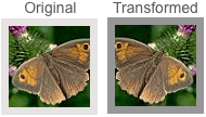
In the flow method, we specify where to save the transformed images. Make sure this directory exists! We also prefix the newly created images for convenience. The flow method would run infinitely, but for this example, we only generate three images. So when our counter reaches this value, we break the for loop. You can see the result below.

Width shift
In the width_shift_range parameter, you specify the ratio of the original width by which the image can be shifted to the left or right. Again, the fill_mode will fill up the newly created empty pixels. For the remaining examples, I will only show how to instantiate the ImageDataGenerator with the respective parameter. The code to generate the images is the same as in the rotation example.
imgGen = ImageDataGenerator(width_shift_range = 90)
In the transformed images we see that the image is shifted to the right. The empty pixels are filled which gives it a bit of a stretched look.
The same can be done for shifting up or down by specifying a value for the height_shift_range parameter.

Rescale
Rescaling an image will multiply the RGB values of each pixel by a chosen value before any other preprocessing. In our example, we apply min-max scaling to the values. As a result, these values will range between 0 and 1. This makes the values smaller and easier for the model to process.
imgGen = ImageDataGenerator(rescale = 1./255)

Shear
With the shear_range parameter, we can specify how the shearing transformations must be applied. This transformation can produce rather weird images when the value is set too high. So don’t set it too high.
imgGen = ImageDataGenerator(shear_range = 0.2)

Zoom
This transformation will zoom inside the picture. Just like the shearing parameter, this value should not be exaggerated to keep the images realistic.
imgGen = ImageDataGenerator(zoom_range = 0.2)
Horizontal flip
This transformation flips an image horizontally. Life can be simple sometimes…
imgGen = ImageDataGenerator(horizontal_flip = True)
All transformations combined
Now that we have seen the effect of each transformation separately, we apply all the combinations together.
imgGen = ImageDataGenerator(
    rotation_range = 40,
    width_shift_range = 0.2,
    height_shift_range = 0.2,
    rescale = 1./255,
    shear_range = 0.2,
    zoom_range = 0.2,
    horizontal_flip = True)
i = 1
for batch in imgGen.flow(x, batch_size=1, save_to_dir='example_transformations', save_format='jpeg', save_prefix='all'):
    i += 1
    if i > 3:
        break

Setting up the folder structure
We need to store these images in a specific folder structure. As such we can use the method flow_from_directory to augment the images and create the corresponding labels. This folder structure needs to look like this:
- train
- maniola_jurtina
- 0.jpg
- 1.jpg
- …
- pyronia_tithonus
- 0.jpg
- 1.jpg
- …
- validation
- maniola_jurtina
- 0.jpg
- 1.jpg
- …
- pyronia_tithonus
- 0.jpg
- 1.jpg
- …
To create this folder structure I created a gist img_train_test_split.py. Feel free to use it in your projects.
Creating the generators
Just as before, we specify the configuration parameters for the training generator. The validation images will not be transformed as the training images. We only divide the RGB values to make them smaller.
The flow_from_directory method takes the images from the train or validation folder and generates batches of 32 transformed images. By setting the class_mode to ‘binary’ a one-dimensional label is created based on the image’s folder name.
train_datagen = ImageDataGenerator(
    rotation_range = 40,
    width_shift_range = 0.2,
    height_shift_range = 0.2,
    rescale = 1./255,
    shear_range = 0.2,
    zoom_range = 0.2,
    horizontal_flip = True)
validation_datagen = ImageDataGenerator(rescale=1./255)
train_generator = train_datagen.flow_from_directory(
    'data/train',
    batch_size=32,
    class_mode='binary')
validation_generator = validation_datagen.flow_from_directory(
    'data/validation',
    batch_size=32,
    class_mode='binary')
What about different image sizes?
The Flickr API lets you download images of specific sizes. However, in real-world applications the image sizes are not always constant. If the aspect ratio of the images is the same, we can simply resize the images. Otherwise, we can crop the images. Unfortunately, it is difficult to crop the image while keeping the object we want to classify intact.
Keras can deal with different image sizes. When configuring the model you can specify None for the width and height in input_shape.
input_shape=(3, None, None)  # Theano
input_shape=(None, None, 3)  # Tensorflow
I wanted to show that it is possible to work with different image sizes, however, it has some drawbacks.
- not all layers (e.g. Flatten) will work with None as an input dimension
- it can be computationally heavy to run
Building the deep learning model
For the remainder of this article, I will discuss the structure of a convolutional neural network, illustrated with some examples for our butterfly project. At the end of this article, we’ll have our first classification results.
What layers does a convolutional neural network consist of?
Of course, you can choose how many layers and their type to add to your convolutional neural network (also called CNN or convnet). In this project we will start with the following structure:

Let’s understand what each layer does and how we create them with Keras.
Input layer
These different versions of the images were modified via several transformations. Then, these images are converted into a numerical representation or a matrix.
The dimensions of this matrix will be width x height x number of (color) channels. For RGB images the number of channels will be three. For grayscale images, this is equal to one. Below you can see a numerical representation of a 7×7 RGB image.

As our images are of size 75×75, we need to specify that in the input_shape parameter when adding the first convolutional layer.
cnn = Sequential()
cnn.add(Conv2D(32,(3,3), input_shape = (3 ,75 ,75)))
Convolutional layer
In the first layers, the convolutional neural network will look for lower-level features, like horizontal or vertical edges. The further we go in the network it will look for higher-level features, such as a wing of a butterfly, for example. But how does it detect features when it gets only numbers as input? That’s where filters come in.
Filters (or kernels)
You can think of a filter as a searchlight of a specific size that scans over the image. The filter example below has dimensions of 3x3x3 and contains weights that will detect a vertical edge. For a grayscale image, the dimensions would have been 3x3x1. Usually, a filter has smaller dimensions than the image we want to classify. 3×3, 5×5 or 7×7 are typically used. The third dimension should always be equal to the number of channels.

While scanning the image, the RGB values are transformed. It does this transformation by multiplying the RGB values with the filter’s weights. Finally, the multiplied values are then summed over all channels. In our 7x7x3 image example and the 3x3x3 filter, this would result in a 5x5x1 outcome.
The animation below illustrates this convolutional operation. For simplicity, we only look for a vertical edge in the Red channel. Thus, the weights for the Green and Blue channels are all equal to zero. But you should keep in mind that the multiplication results for these channels are added to the result of the Red channel.
As shown below the convolutional layer will produce numerical outcomes. When you have higher numbers, this means that the filter came across the feature it was looking for. In our example, a vertical edge.

We can specify that we want more than one filter. These filters could have their own feature to look for in an image. Suppose we use 32 filters of size 3x3x3. The result of all filters is stacked and we end up with a 5x5x32 volume in our example. In the code snippet above we added 32 filters of size 3x3x3.
Stride
In the example above we saw that the filter moves up one pixel at a time. This is the so-called stride. We could increase the number of pixels the filter moves up. Increasing the stride will reduce the dimensions of the original image much faster. In the example below, you see how the filter moves around with a stride of 2, which would result in a 3x3x1 outcome for a 3x3x3 filter and a 7x7x3 image.
Padding
By applying a filter, the dimensions of the original image are quickly reduced. Especially the pixels at the edges of the image are only used once in the convolutional operation. This results in a loss of information. If you want to avoid that, you can specify padding. Padding adds “extra pixels” around the image.
Suppose we add padding of one pixel around the 7x7x3 image. This results in a 9x9x3 image. If we apply a 3x3x3 filter and a stride of 1, we end up with a 7x7x1 outcome. So, in that case, we preserve the dimensions of the original image and the outer pixels are used more than once.
You can calculate the resulting outcome of the convolutional operation with specific padding and stride as follows:
1 + [(original dimension + padding x 2 — filter dimension) / stride size]
For example, suppose we have this set-up of our conv layer:
- 7x7x3 image
- 3x3x3 filter
- padding of 1 pixel
- stride of 2 pixels
That will give 1 + [(7 + 1 x 2–3) / 2] = 4
Why do we need convolutional layers?
A benefit of using conv layers is that the number of parameters to estimate is much lower. Much lower compared to having a normal hidden layer. Suppose we continue with our example image of 7x7x3 and a filter of 3x3x3 with no padding and stride of 1. The convolutional layer would have 5x5x1 + 1 bias = 26 weights to estimate. In a neural network with 7x7x3 inputs and 5x5x1 neurons in the hidden layer, we would need to estimate 3.675 weights. Imagine what this number is when you have larger images…
ReLu layer
Or Rectified Linear unit layer. This layer adds nonlinearity to the network. The convolutional layer is a linear layer as it sums up the multiplications of the filter weights and RGB values.
The outcome of a ReLu function is equal to zero for all values of x <= 0. Otherwise, it is equal to the value of x. The code in Keras to add a ReLu layer is:
cnn.add(Activation(‘relu’))
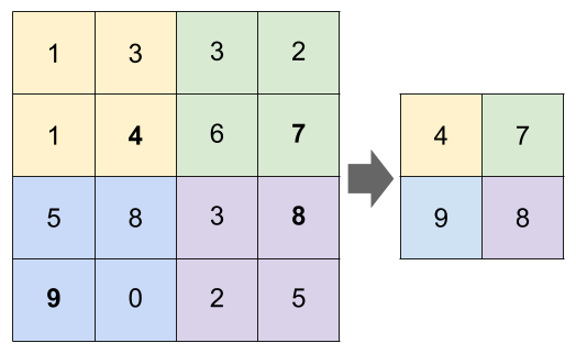
Pooling
Pooling aggregates the input volume in order to reduce the dimensions further. This speeds up computation time as the number of parameters to be estimated are reduced. Besides that, it helps to avoid overfitting by making the network more robust. Below we illustrate max pooling with a size of 2×2 and stride of 2.
The code in Keras to add pooling with a size of 2×2 is:
cnn.add(MaxPooling2D(pool_size = (2 ,2)))
Fully connected layer
At the end, the convnet is able to detect higher level features in the input images. This can then serve as an input for a fully connected layer. Before we can do that, we will flatten the output of the last ReLu layer. Flattening means we convert it to a vector. The vector values are then connected to all neurons in the fully connected layer. To do that in Python we use the following Keras functions:
cnn.add(Flatten())
cnn.add(Dense(64))
Dropout
Just like pooling, dropout can help to avoid overfitting. It randomly sets a specified fraction of the inputs to zero, during the training of the model. A dropout rate between 20 and 50% is considered to work well.
cnn.add(Dropout(0.2))
Sigmoid activation
Because we want to produce a probability that the image is one of two butterfly species (i.e. binary classification), we can use a sigmoid activation layer.
cnn.add(Activation('relu'))
cnn.add(Dense(1))
cnn.add(Activation( 'sigmoid'))
Applying the convolutional neural network on the butterfly images
Now we can define the complete convolutional neural network structure as displayed at the beginning of this post. First, we need to import the necessary Keras modules. Then we can start adding the layers that we explained above.
from keras.models import Sequential
from keras.layers import Conv2D, MaxPooling2D
from keras.layers import Activation, Flatten, Dense, Dropout
from keras.preprocessing.image import ImageDataGenerator
import time
IMG_SIZE = # Replace with the size of your images
NB_CHANNELS = # 3 for RGB images or 1 for grayscale images
BATCH_SIZE = # Typical values are 8, 16 or 32
NB_TRAIN_IMG = # Replace with the total number training images
NB_VALID_IMG = # Replace with the total number validation images
I made some additional parameters explicit for the conv layers. Here is a short explanation:
- kernel_size specifies the filter size. So for the first conv layer this is size 2×2
- padding = ‘same’ means applying zero padding as such the original image size is preserved.
- padding = ‘valid’ means we do not apply any padding.
- data_format = ‘channels_last’ is just to specify that the number of color channels is specified last in the input_shape argument.
cnn = Sequential()
cnn.add(Conv2D(filters=32,
               kernel_size=(2,2),
               strides=(1,1),
               padding='same',
               input_shape=(IMG_SIZE,IMG_SIZE,NB_CHANNELS),
               data_format='channels_last'))
cnn.add(Activation('relu'))
cnn.add(MaxPooling2D(pool_size=(2,2),
                     strides=2))
cnn.add(Conv2D(filters=64,
               kernel_size=(2,2),
               strides=(1,1),
               padding='valid'))
cnn.add(Activation('relu'))
cnn.add(MaxPooling2D(pool_size=(2,2),
                     strides=2))
cnn.add(Flatten())
cnn.add(Dense(64))
cnn.add(Activation('relu'))
cnn.add(Dropout(0.25))
cnn.add(Dense(1))
cnn.add(Activation('sigmoid'))
cnn.compile(loss='binary_crossentropy', optimizer='rmsprop', metrics=['accuracy'])
Finally, we compile this network structure and set the loss parameter to binary_crossentropy which is good for binary targets and use accuracy as the evaluation metric.
After having specified the network structure, we create the generators for the training and validation samples. On the training samples, we apply data augmentation as explained above. On the validation samples, we do not apply any augmentation as they are just used to evaluate the model performance.
train_datagen = ImageDataGenerator(
    rotation_range = 40,
    width_shift_range = 0.2,
    height_shift_range = 0.2,
    rescale = 1./255,
    shear_range = 0.2,
    zoom_range = 0.2,
    horizontal_flip = True)
validation_datagen = ImageDataGenerator(rescale = 1./255)
train_generator = train_datagen.flow_from_directory(
    '../flickr/img/train',
    target_size=(IMG_SIZE,IMG_SIZE),
    class_mode='binary',
    batch_size = BATCH_SIZE)
validation_generator = validation_datagen.flow_from_directory(
    '../flickr/img/validation',
    target_size=(IMG_SIZE,IMG_SIZE),
    class_mode='binary',
    batch_size = BATCH_SIZE)
With the flow_from_directory method on the generators we can easily go through all the images in the specified directories.
Lastly, we can fit the convolutional neural network on the training data and evaluate with the validation data. The resulting weights of the model can be saved and reused later on.
start = time.time()
cnn.fit_generator(
    train_generator,
    steps_per_epoch=NB_TRAIN_IMG//BATCH_SIZE,
    epochs=50,
    validation_data=validation_generator,
    validation_steps=NB_VALID_IMG//BATCH_SIZE)
end = time.time()
print('Processing time:',(end - start)/60)
cnn.save_weights('cnn_baseline.h5')
The number of epochs is arbitrarily set to 50. An epoch is the cycle of forward propagation, checking the error and then adjusting the weights during backpropagation.
The steps_per_epoch is set to the number of training images divided by the batch size (by the way, the double division symbol will make sure the result is an integer and not a float). Specifying a batch size greater than 1 will speed up the process. Idem for the validation_steps parameter.
Results
After running 50 epochs, we have a training accuracy of 0.8091 and validation accuracy of 0.7359. So the convolutional neural network still suffers from quite some overfitting. We also see that the validation accuracy varies quite a lot. This is because we have a small set of validation samples. It would be better to do k-fold cross-validation for each evaluation round. But that would take quite some time.
To address the overfitting we could:
- increase the dropout rate
- apply dropout at each layer
- find more training data
We’ll look into the first two options and monitor the result. The results of our first model will serve as a baseline. After applying an extra dropout layer and increasing the dropout rates, the model is a bit less overfitted.

I hope you’ve all enjoyed reading this post and learned something new. The full code is available on Github. Cheers!