Deep Learning Tutorial – How to Use PyTorch and Transfer Learning to Diagnose COVID-19 Patients

Ever since the outbreak of COVID-19 in December 2019, researchers in the field of artificial intelligence and machine learning have been trying to find better ways to diagnose the disease.

They've worked on developing algorithms that would detect the disease within a matter of seconds – and only by looking at chest X-rays and/or CT scan images.

Some of these techniques have proven to be extremely useful and accurate in diagnosing COVID-19 cases.

There are multiple approaches that use both machine and deep learning to detect and/or classify of the disease. And researches have proposed newly developed architectures along with transfer learning approaches.

In this article, we will look at a transfer learning approach that classifies COVID-19 cases using chest X-ray images.

The model we are going to use is one of the seven variants of the EfficientNet architecture. We will use a pre-trained model on the immense ImageNet dataset. EfficientNet is an advanced and complex convolutional neural network-based architecture.

We will further investigate the details of Convolutional Neural Networks, pre-trained models, and EfficientNet during the course of this article. I've divided it into five parts:

1. What are convolutional neural networks?
2. A dive into transfer learning.
3. What is EfficientNet?
4. An introduction to PyTorch.
5. Implementation of COVID-19 classifier using EfficientNet with PyTorch.

This tutorial assumes that you have prior knowledge of both machine learning and deep learning. If you want to further develop your foundation in these topics, check out this article on Artificial Intelligence vs Machine Learning vs Deep Learning.

Also, although the dataset we'll work with here is COVID-related, you can apply the actual code implementation and analysis to other datasets.

What is a Convolutional Neural Network?

Convolutional Neural networks (CNNs) are a type of deep neural network that works on visual data – this is, images. A CNN takes an image as an input and performs two or three-dimensional convolutional operations on the image with several filters, also referred to as kernels.

These convolution operations output a 2D or 3D matrix which contains the learnable weights and biases regarding the spatial information of the input image. This output matrix is referred to as the feature map of the image.

Processing a convolutional neural network in the training process can be, in some cases, extremely slow. This is why it's a good idea to use GPUs and TPUs during training for deep learning techniques, especially convolutional neural networks.

Convolutional neural networks learn spatial and temporal information about the image far better than the basic feed forward neural network. Also, CNNs can reduce the size of the image while retaining the most important information in the image, which is crucial for predictive analysis of images.

The starting layers of convolutional neural networks learn the abstract and simpler features in an image, such as lines and edges. But as we move deeper into the network, the feature map turns to the more complex structures in the image.

It starts to learn the more specific features of the image, such as a cat, a dog, or a person, the same way we would, as humans, perceive the world around us. This is a core concept in modern deep learning-based computer vision.

Now before we move on to advanced concepts, it is important to learn the basics of 2D convolution.

What is 2D Convolution?

2D convolution is a bit complex to explain, but here it goes: if the convolutional process (which is extensively used in h1-D signal processing) is performed between two signals – but not just along a single dimension, rather along two mutually perpendicular dimensions – it is called 2D convolution.

In the case of images, the two mutually perpendicular dimensions are the rows and columns of a greyscale image. The convolutional operation is mathematically done by multiplying and then accumulating the values of the overlapping samples of the two input signals, where one of the signals is flipped. The output of this multiplication and accumulation gives a single point on the feature map.

In the case of CNNs, the image is one signal and the filter/kernel is the second signal which is flipped. The size of the kernel is always smaller than that of the image.

The flipped kernel is then swept across the whole image both row by row and column by column to output the feature map.

Here a 3x3 kernel is swept across a 6x6 image to output a 4x4 feature map. As you can see, the dimensions of the output feature map are smaller than the input image. So there are a few concepts used in convolution to control the dimensions of the output feature map. These include padding, stride, and kernel size.

Padding is the manual addition of rows and columns around the input to keep the output dimension the same as the input dimension or vary it.

Stride refers to the jump the kernel takes during the sweep, both in columns and rows. In the example above, the stride of the convolution is 1 as the kernel is moving one unit in both rows and columns.

Kernel size refers to the dimensions of the kernel used. Changing the dimensions of the kernel to be swept changes the output size of the feature map.

The image below describes the convolution with the same kernel size but with a padding of 1 and stride of 2.

The equation that describes the relationship of stride, padding, and kernel size to input and output dimensions is as follows:

The concept of 3D convolution is just an extension of 2D convolution where both the input image and the kernel are three-dimensional.

Like 2D convolution, we sweep the three-dimensional kernel across the whole image in two mutually perpendicular dimensions, namely the rows and the columns.

We do not usually sweep the kernel across the color channels because the kernel has the same third dimension, that is the channel length, as the original image. This gives an output feature map that is two-dimensional instead of three.

To learn more about the details of 3D convolution, you can read this article.

What is Transfer Learning?

In transfer learning, you take a machine or deep learning model that is pre-trained on a previous dataset and use it to solve a different problem without needing to re-train the whole model.

Instead, you can just use the weights and biases of the pre-trained model to make a prediction. You transfer the weights from one model to your own model and adjust them to your own dataset without re-training all the previous layers of the architecture.

We use transfer learning in the applications of convolutional neural networks and natural language processing because it decreases the computation time and complexity of the training process. And, in many cases, it performs surprisingly well.

This also helps in cases where we have limited data available – since neural networks demand an extremely large amount of data to achieve good performance.

This means that using transfer learning methods can greatly reduce the demand for data since the weights and biases are pre-adjusted and are able to work better with just a small amount of data by tweaking the weights and biases a little.

But transfer learning models do not always give you great performance (although the newer architectures perform efficiently on almost every problem). Still, sometimes the problem at hand needs an architecture that is pre-trained on data that's similar to what you have. This factor depends upon the complexity of the problem you are trying to solve.

There are a couple ways you can perform transfer learning:

1. Using a pre-trained model.
2. Developing a new model.

You can use a pre-trained model in two ways. First, you can use the pre-trained weights and biases as initial parameters for your own model, and then train a whole convolutional model using those weights.

The other way is to perform feature extraction from the pre-trained model. You use the parameters of the pre-trained model to extract features from your input image and just train a simple classifier on top of it.

Another option is that if you have a problem with a small amount of data, you develop another model for a similar problem that has a large amount of data and train the model. Then you can use the trained weights from the new model to solve the original problem with less data.

In this tutorial, we will be using a pre-trained model as a feature extractor and we'll train a simple classifier on top of it to output the prediction.

There are many well-known architectures in the field of deep learning that are nowadays used for the purpose of transfer learning. Almost all of these are trained on the ImageNet dataset which is the largest open-source dataset available. It contains around 1000 classes and has around fifteen million instances.

Among these pre-trained architectures, LeNet is the first one that was proposed in 1998. Other well-known models include VGG, ResNet, AlexNet, GoogleNet, Inception, and Xception.

EfficientNet is also part of the series that was proposed recently, in 2019.

What is EfficientNet?

EfficientNet (or perhaps it's better to say EfficientNets) is a family of convolutional neural network-based image classification models. They perform extremely well on the state-of-the-art ImageNet dataset and other popular datasets such as CIFAR-100 and Flowers.

In addition to performing so well, the architecture is small and computes faster than any of the previous models. The architecture has variants ranging from EfficientNet-B0 up to EffieicntNet-B7.

The variants ranging from B0 to B7 are based on the compound scaling method to scale up the baseline in B0 to obtain B1 to B7. EfficientNet-B7 acquired a Top-1 accuracy of 84.4% on the ImageNet dataset, which is the highest level of Top-1 accuracy ever achieved on ImageNet.

If you want to learn more about how EfficientNets work, you can read this paper ‘Efficientnet: Rethinking Model Scaling for Convolutional Neural Networks.’

In the coding tutorial further along in this article, we'll be using the EfficientNet-B0 as a feature extractor and a classifier on top of it to classify COVID-19 using chest x-ray images.

An Introduction to PyTorch

PyTorch is a Python-supported library that helps us build deep learning models. Unlike Keras (another deep learning library), PyTorch is flexible and gives the developer more control.

It is similar to NumPy in processing but has a faster GPU acceleration. To learn more about NumPy and its features, you can check out this in-depth guide along with its documentation.

PyTorch has a data structure known as a ‘Tensor’ that is similar to the NumPy ndarray but it has the option to operate on GPU.

PyTorch provides an uncomplicated way to switch computation between a CPU and a GPU. It also supports processing on NumPy arrays by simply providing a built-in module that can convert NumPy arrays into Tensors and vice versa.

One of the handiest modules in PyTorch is grad(). It allows you to compute the gradient of a tensor as it goes forward into processing without needing to manually compute the gradient and store it.

This gives you greater control of your deep learning operations, specifically back propagation, during the training process. This is helpful when computing the loss function which lets you adjust the parameters of a model.

We can also limit a tensor so that its gradient is not computed during the entire process by making the module's requires_grad equal False. To learn more about tensors and how to perform gradient computations in PyTorch, you can check out this tutorial and this course.

How to Implement a COVID-19 Classifier using EfficientNet with PyTorch

Now let's move on to the practical implementation of EfficientNet in PyTorch. We will use the B0 variant of the EfficientNet family.

First, we'll examine the data and preprocess it. Kaggle has an vast library of datasets available for open-source use in projects and research. There are no limits as to what dataset can be used for this project. You can use any dataset containing chest X-ray images of COVID-19 patients and people without COVID.

For the sake of this tutorial, we'll use this dataset here. But for the code to work on your custom dataset, you must divide your data into three directories: train, test, and valid.

Each directory should contain two more directories with the labels covid and normal. These covid and normal folders will contain the images corresponding to the specific class of the directory they are present in.

The original dataset we'll use in this article contains three folders: covid, normal, and pneumonia. We discard the pneumonia folder completely and divide the other data in the same way described above.

We do this to create a logical division between the data used for training and the data used for testing and validation. Also, PyTorch, by default, takes the name of the folder, an instance it is present in, as the label of the class – so we do not have a label file corresponding to the input dataset.

The data and the architecture

Let's have a look at the data. Below we can see the x-ray images of patients with COVID-19:

And here we can see the normal category’s x-ray images:

There are 237 total layers in the B-0 architecture. The whole architecture can be condensed into the following diagrams. We provide the x-ray data to the input layer.

We will freeze the learning of the weights across all these blocks as we will be using the pre-trained weights to extract the features from our own input.

We'll do the feature extraction after the input passes Module 7. We then transfer the feature map obtained from Module 7 to our own final classification layers (this is why it's called transfer learning). We top the architecture with the following top layers:

• BatchNorm1d
• Linear(output neurons = 512)
• ReLU()
• BatchNorm1d()
• Linear(output neurons = 128)
• ReLU()
• BatchNorm1d()
• Dropout(probability of zeroing the parameters = 0.4)
• Linear(output neurons = 2)

Let's head over to the code

Now before we start the code, there are a couple of dependencies we need to install. First, you'll need to install PyTorch on your local machine. You can do this using the pip install command in your Python environment. Refer here to install it depending on your machine (whether it has GPU available or not).

Before you move on to the code, I strongly recommend that you actually work through the code yourself. This makes it much easier to understand. With that said, you can access the full code in a Jupyter notebook here.

You also need to install Efficientnet support for PyTorch into the same Python environment. Run the command below to install it:

pip install efficientnet_pytorch

Apart from this you will need to import some other dependencies at the start of the code.

Now we start building the classification model. To start, we import all the necessary modules:

#importing required modules
import gdown
import zipfile
import numpy as np
from glob import glob
import matplotlib.pyplot as plt
import torch
import torch.nn as nn
from torchsummary import summary
from torchvision import datasets, transforms as T
from efficientnet_pytorch import EfficientNet
import os
import torch.optim as optim
from PIL import ImageFile
from sklearn.metrics import accuracy_score

All these modules are essential to perform multiple functions across the model. You can install all the absent modules using the pip command.

Then we download and extract the data we prepared for the model:

#importing data
#Dataset address
url = 'https://drive.google.com/uc?export=download&id=1B75cOYH7VCaiqdeQYvMuUuy_Mn_5tPMY'
output = 'data.zip'
gdown.download(url, output, quiet=False)
#giving zip file name
data_dir='./data.zip'
#Extracting data from zip file
with zipfile.ZipFile(data_dir, 'r') as zf:
zf.extractall('./data/')

The gdown.download module downloads the data from the URL provided and the zipfile.extractall extracts the data into the same directory where you currently are (or the same runtime if you are working on Google Colab).

I highly recommend working on Google Colab for this project in case you do not locally have a GPU available.

Next, create a check variable to check the availability of a GPU.

#Checking the availability of a GPU
use_cuda = torch.cuda.is_available()

This module returns ‘True’ if GPU is available and ‘False' if not.

Next, we need to apply pre-processing techniques to the data. Since our data is pre-augmented, we do not need to apply many pre-processing techniques to it. We only resize all the images to a single size of (224,224). We do this because the images in our dataset are all of different dimensions and we need a consistent dimension for the model.

We'll also convert the images to tensors to be processed by PyTorch and then we normalize all the images. This normalize function normalizes all the images with a mean and standard deviation of 0.5.

After that, we create the locations for the train, test and validation sets which will be given as input to the ‘datasets’ module. We do this so that the PyTorch model knows exactly where the data is located and also so that that data can be loaded to the GPU. We keep a batch size of 32.

#declaring batch size
batch_size = 32

#applying required transformations on the dataset
img_transforms = {
    'train':
    T.Compose([
        T.Resize(size=(224,224)), 
        T.ToTensor(),
        T.Normalize([0.5, 0.5, 0.5], [0.5, 0.5, 0.5]), 
        ]),

    'valid':
    T.Compose([
        T.Resize(size=(224,224)),
        T.ToTensor(),
        T.Normalize([0.5, 0.5, 0.5], [0.5, 0.5, 0.5])
        ]),

    'test':
    T.Compose([
        T.Resize(size=(224,224)),
        T.ToTensor(),
        T.Normalize([0.5, 0.5, 0.5], [0.5, 0.5, 0.5])
        ]),
     }

# creating Location of data: train, validation, test
data='./data/'

train_path=os.path.join(data,'train')
valid_path=os.path.join(data,'test')
test_path=os.path.join(data,'valid')


# creating Datasets to each of  folder created in prev
train_file=datasets.ImageFolder(train_path,transform=img_transforms['train'])
valid_file=datasets.ImageFolder(valid_path,transform=img_transforms['valid'])
test_file=datasets.ImageFolder(test_path,transform=img_transforms['test'])


#Creating loaders for the dataset
loaders_transfer={
    'train':torch.utils.data.DataLoader(train_file,batch_size,shuffle=True),
    'valid':torch.utils.data.DataLoader(valid_file,batch_size,shuffle=True),
    'test': torch.utils.data.DataLoader(test_file,batch_size,shuffle=True)
}

After pre-processing, we move on to building the model.

#importing the pretrained EfficientNet model

model_transfer = EfficientNet.from_pretrained('efficientnet-b0')

# Freeze weights
for param in model_transfer.parameters():
    param.requires_grad = False
in_features = model_transfer._fc.in_features


# Defining Dense top layers after the convolutional layers
model_transfer._fc = nn.Sequential(
    nn.BatchNorm1d(num_features=in_features),    
    nn.Linear(in_features, 512),
    nn.ReLU(),
    nn.BatchNorm1d(512),
    nn.Linear(512, 128),
    nn.ReLU(),
    nn.BatchNorm1d(num_features=128),
    nn.Dropout(0.4),
    nn.Linear(128, 2),
    )
if use_cuda:
    model_transfer = model_transfer.cuda()

First, we import the EfficientNet-B0 model with its pre-trained weights. Next, we disable the training of the parameters of the model because we are going to use the pre-trained parameters to extract features from our data.

Then we replace the top fully connected layers of the model with our own classifier.

Batchnorm normalizes the whole batch of data into the number of neurons given as an argument. This reduces the complexity of the model and prevents it from overfitting. Dropout does something similar – it zeroes out some neurons in the model with a probability of the value given as an argument.

The Linear layer is a simple fully-connected neural network layer.

Finally, we transfer our model to the GPU, if available.

# selecting loss function
criterion_transfer = nn.CrossEntropyLoss()

#using Adam classifier
optimizer_transfer = optim.Adam(model_transfer.parameters(), lr=0.0005)

Here, we select the loss function and the optimizer for our training phase. We also define the value of the learning rate for the optimizer. You can change this value to see how different learning rates influence the model in different ways.

Next, we move on to the training of the model.

ImageFile.LOAD_TRUNCATED_IMAGES = True

# Creating the function for training
def train(n_epochs, loaders, model, optimizer, criterion, use_cuda, save_path):
    """returns trained model"""
    # initialize tracker for minimum validation loss
    valid_loss_min = np.Inf 
    trainingloss = []
    validationloss = []

    for epoch in range(1, n_epochs+1):
        # initialize the variables to monitor training and validation loss
        train_loss = 0.0
        valid_loss = 0.0
        
        ###################
        # training the model #
        ###################
        model.train()
        for batch_idx, (data, target) in enumerate(loaders['train']):
            # move to GPU
            if use_cuda:
                data, target = data.cuda(), target.cuda()
          
            optimizer.zero_grad()
            output = model(data)
            loss = criterion(output, target)
            loss.backward()
            optimizer.step()
           
            train_loss = train_loss + ((1 / (batch_idx + 1)) * (loss.data - train_loss))
    
        ######################    
        # validating the model #
        ######################
        model.eval()
        for batch_idx, (data, target) in enumerate(loaders['valid']):
            if use_cuda:
                data, target = data.cuda(), target.cuda()
            
            output = model(data)
            loss = criterion(output, target)
            valid_loss = valid_loss + ((1 / (batch_idx + 1)) * (loss.data - valid_loss))
        
        train_loss = train_loss/len(train_file)
        valid_loss = valid_loss/len(valid_file)

        trainingloss.append(train_loss)
        validationloss.append(valid_loss)

        # printing training/validation statistics 
        print('Epoch: {} \tTraining Loss: {:.6f} \tValidation Loss: {:.6f}'.format(
            epoch, 
            train_loss,
            valid_loss
            ))
        
        ## saving the model if validation loss has decreased
        if valid_loss < valid_loss_min:
            torch.save(model.state_dict(), save_path)
            
            valid_loss_min = valid_loss
            
    # return trained model
    return model, trainingloss, validationloss

We create a function for the training and validation phase of the model. We allow the model to accept truncated images also with fewer than three channels. We initialize the values of the train and validation losses and start the training loop. We import the data batch by batch from the data loaders and perform the training operations.

After the training loop, we start the validation loop where we only compute the loss and the output predictions and do not update the parameters as we did in the training loop. We save the model which has the minimum loss for the validation set.

# training the model

n_epochs=10

model_transfer, train_loss, valid_loss = train(n_epochs, loaders_transfer, model_transfer, optimizer_transfer, criterion_transfer, use_cuda, 'model.pt')

We run the model for 10 epochs, that is 10 loops. You can change the number of epochs and test out the loss values. The saved model is saved under the name model.pt. Now we load the model and move on to the testing phase.

# Defining the test function

def test(loaders, model, criterion, use_cuda):

    # monitoring test loss and accuracy
    test_loss = 0.
    correct = 0.
    total = 0.
    preds = []
    targets = []

    model.eval()
    for batch_idx, (data, target) in enumerate(loaders['test']):
        # moving to GPU
        if use_cuda:
            data, target = data.cuda(), target.cuda()
        # forward pass
        output = model(data)
        # calculate the loss
        loss = criterion(output, target)
        # updating average test loss 
        test_loss = test_loss + ((1 / (batch_idx + 1)) * (loss.data - test_loss))
        # converting the output probabilities to predicted class
        pred = output.data.max(1, keepdim=True)[1]
        preds.append(pred)
        targets.append(target)
        # compare predictions
        correct += np.sum(np.squeeze(pred.eq(target.data.view_as(pred))).cpu().numpy())
        total += data.size(0)
    
    return preds, targets

# calling test function
preds, targets = test(loaders_transfer, model_transfer, criterion_transfer, use_cuda)

We now create a test function to apply our model to our test dataset and evaluate its performance.

We pass the dataset batch by batch as we did in the train and testing phase, but we only do it once here instead of 10 epochs. This is because we just have to test the model and not update the parameters.

The function returns the predictions it computed for the input test set and also the original target values of the test set.

Now we compute the accuracy of the model. First, we need to convert the tensors, that is predictions and targets, into NumPy arrays. We do this by first moving them from the GPU to the CPU and then converting them to NumPy arrays. The following code does this:

#converting the tensor object to a list for metric functions

preds2, targets2 = [],[]

for i in preds:
  for j in range(len(i)):
    preds2.append(i.cpu().numpy()[j])
for i in targets:
  for j in range(len(i)):
    targets2.append(i.cpu().numpy()[j])

Now we compute the accuracy using the accuracy metric of the sklearn library.

#Computing the accuracy
acc = accuracy_score(targets2, preds2)
print("Accuracy: ", acc)

Our model had an accuracy of 95.45%.

The next image is the confusion matrix for the test run of the classifier. In it, you can see the visual of the model’s performance. The actual labels indicate whether the person had COVID or not, while the predicted labels indicate how our model classified the images.

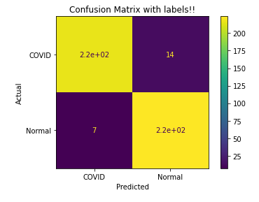
As we can see, our model predicted most of the labels correctly. The small portion of wrongly predicted labels include 7 people who did not have COVID, but our model predicted they did. This is not too alarming.

On the other hand, there were 14 examples where our model predicted that they did not have COVID, but they did. In machine learning, these are called false negatives. This is a very alarming situation because we would've sent home people suffering from COVID-19. This would increase their risk that the disease would get worse.

Conclusion

Convolutional neural networks have proved extremely useful in computer vision techniques, and we can also use them efficiently in medical imaging and diagnosis.

Transfer learning is an effective method for using pre-trained architectures to perform efficiently in other applications.

But as we saw above, using these models depends upon what kind of problem we have and what our objectives are. Just like in the detection of COVID-19, we would prefer to have a model that gives us 0 false negatives. But there's still great potential for deep learning to be useful in COVID diagnosis as well as other medical diagnosis techniques.

Thanks for reading! If you enjoyed the article and would like to read more interesting articles around computer science, Python and JavaScript, please follow me on Twitter.