

I've been using Microsoft Excel and Google Sheets in my business for over a decade. And as I've learned better ways to clean and validate data, it's increased productivity, decreased human errors, and generally caused a lot of joy! 🥳
In this article, we'll look at two ways to validate and/or apply conditional formatting to a sample order form to prevent errors and speed up fulfillment.
 gif of man saying, "there is no room for error"
You can find the Excel sheet we're using for this tutorial here.
You may download a local copy to tinker with by selecting File, Save As, Download a Copy:
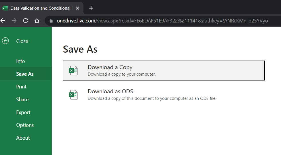 Download a copy of Excel Workbook
You can find a Google Sheets version of the same thing here.
You may download or make a copy online by selecting File, Download or File, Make a copy.
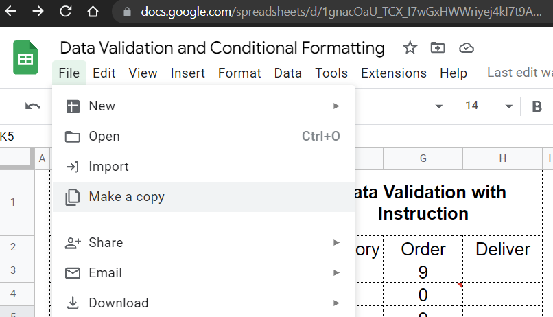 Download or make a copy of Google Sheet
I'll discuss the Excel version from here on, making reference when something differs in Google Sheets.
Video Walkthrough
Oh, and here's an enjoyable video walkthrough should you feel so inclined. 😁😁
Setup
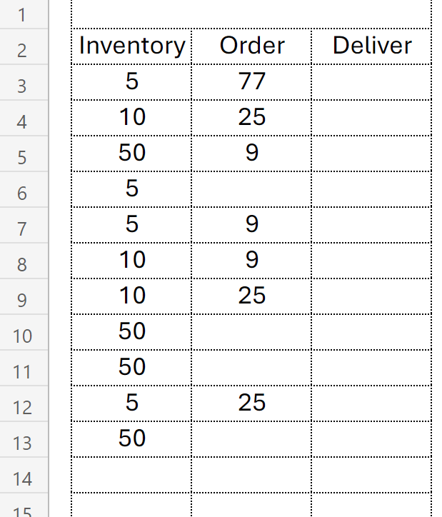
I've created a three column order form where a store may inventory their product and enter an amount to order. The third column is used by the warehouse to enter how many were actually delivered. This is a real world setup that we'll use in simplified form for this tutorial.
 Sample order form in Excel
It can be difficult for fulfillment if there are zeros entered into the order column. Instead of allowing this, we'll use a couple tools to show how to control values in a cell. No matter how clear the directions are, someone will always forget and enter a zero.
Conditional Formatting
By applying conditional formatting, we can effectively white-out the cells that contain zeros (or any negative values).
From the Home Ribbon in Excel and the Format menu in Google Sheets, select Conditional Formatting.
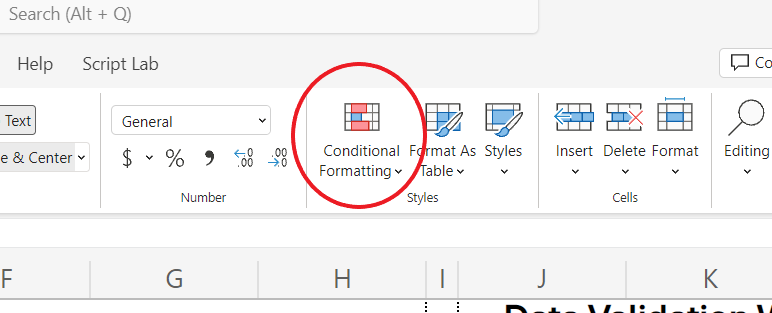
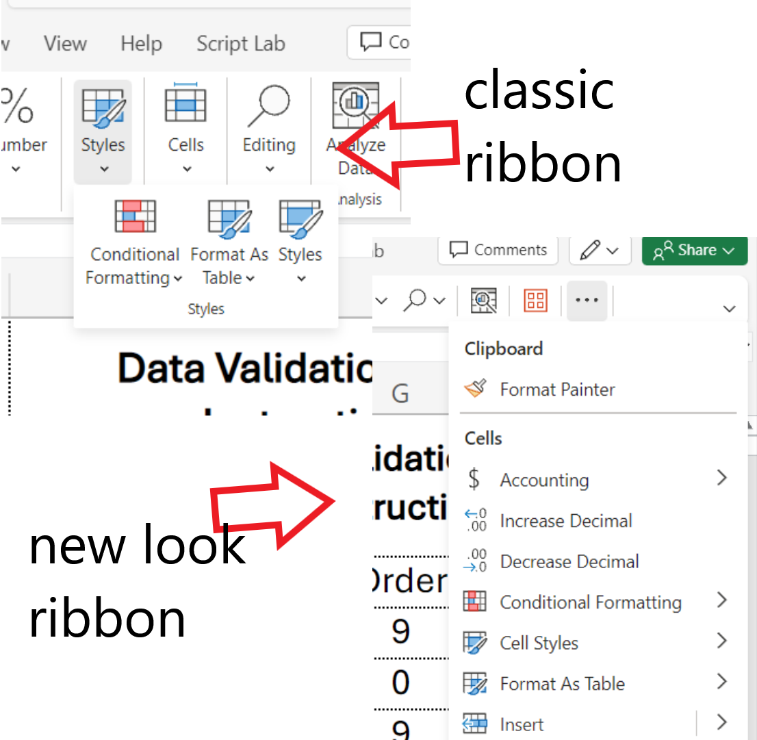
If you don't see the conditional formatting as an option, it'll be over in the styles dropdown or in the far right in a three-dotted dropdown, depending on whether you've got the classic or the new style of ribbon displayed.
 Conditional formatting menu in Excel Ribbons
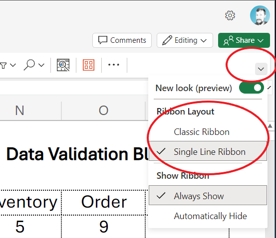
If you want to change your ribbon's layout, select this dropdown arrow at the far right of the ribbon:
 Change Excel Ribbon layout
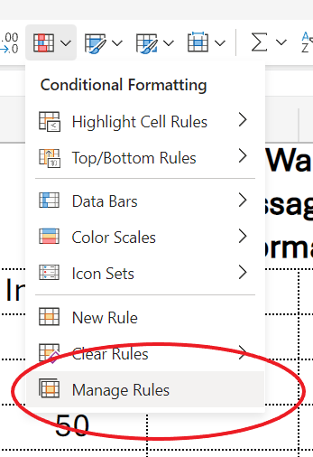
Once you're in the conditional format menu, click Manage Rules. This will let you specify the formatting depending on a ton of options.
 Manage conditional formatting rules in Excel
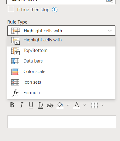
This is where Microsoft Excel does have a leg up on Google Sheets. Excel has more options laid out in a more intuitive way. You can do the same things in each program, but Excel has organized theirs a little better in my opinion.
 Conditional formatting menu organization in Excel
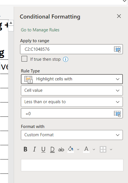
We are going to select the Order column as our range and then highlight cells with cell values of less than or equals to zero.
At other times, you'll be using conditional formatting to make data visualization using colors and color scales, but in our case, we want to blot out the zero value.
To do this, I've simply selected a white fill color and a white text color. 🤔
 Conditional formatting menu
And now, voilà! If a zero amount is entered, it will simply white out to not distract from the fulfillment center:
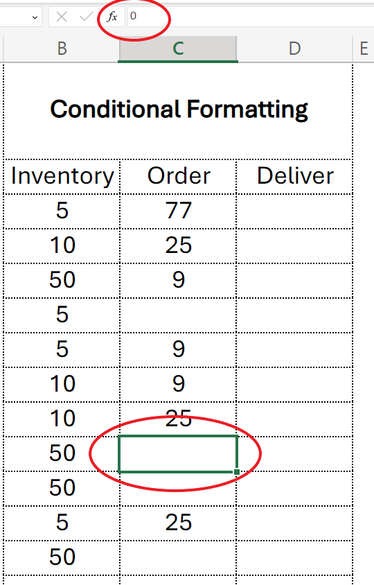 Zero value entered and conditional formatting applied
Data Validation
The second option at our disposal is data validation. You can find this on the data tab in the ribbon, and if you're not seeing it, you can find it by exploring the same ribbon options I detailed above.
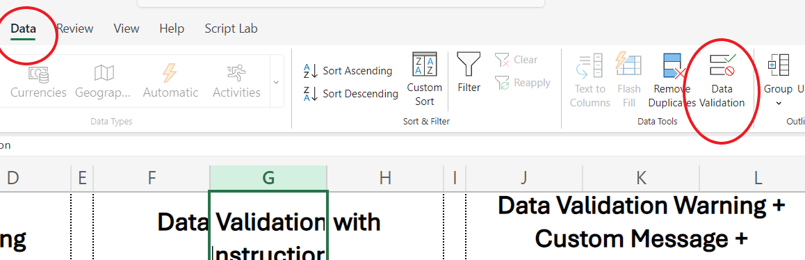 Data validation menu in ribbon
This will give us a host of options to select to validate the data going into a specified range. There are many options to choose from for our data.
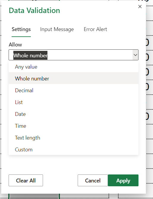
In our case, we want to make sure they are whole numbers greater than zero. Sort of the opposite of the conditional formatting we did above.
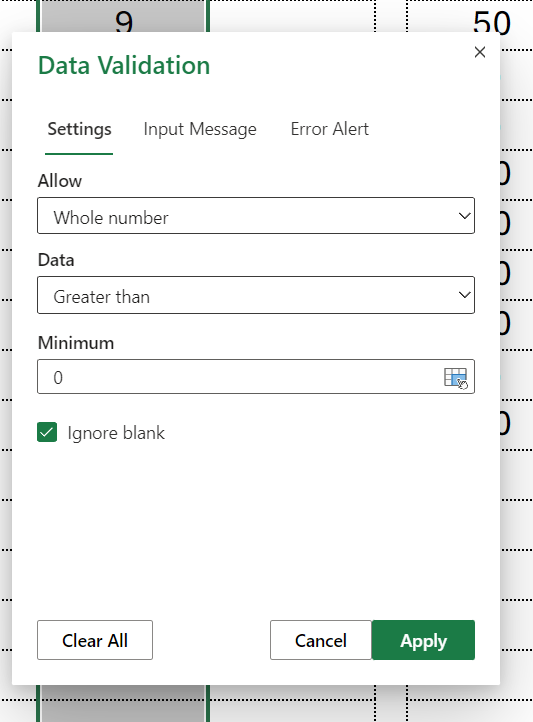 Data validation
Another nice Excel feature that's missing at the time of this writing in Google Sheets is the ability to put an Input Message into the data validation.
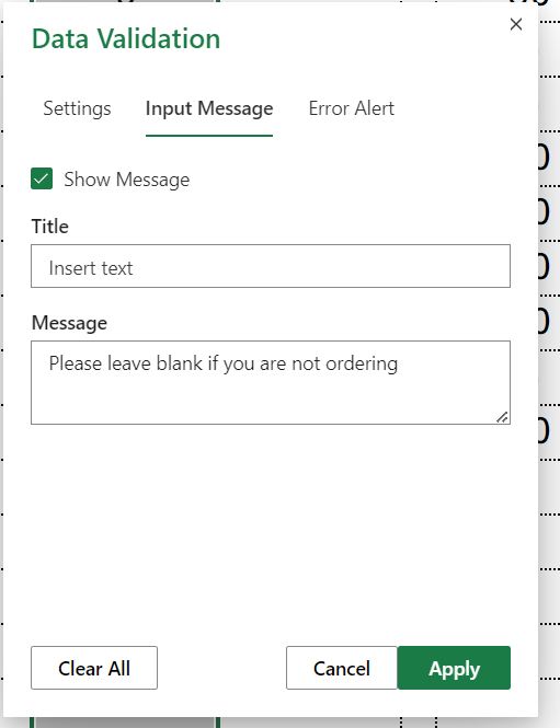 Input message in data validation
Now, whenever you are on cell in the data validation range, a friendly box will pop up with directions reminding you to not order a zero amount. 😀
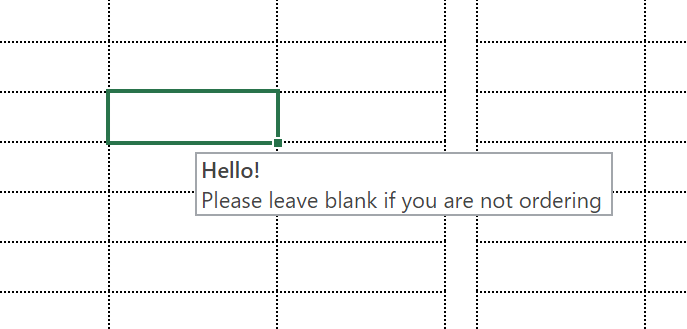 Example of input text in spreadsheet
Data validation in Excel defaults to blocking any input that doesn't adhere to the defined conditions.
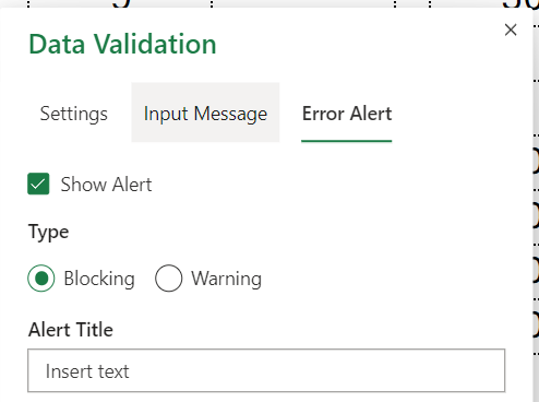
So, you'll receive an ugly pop up preventing you from entering a zero.
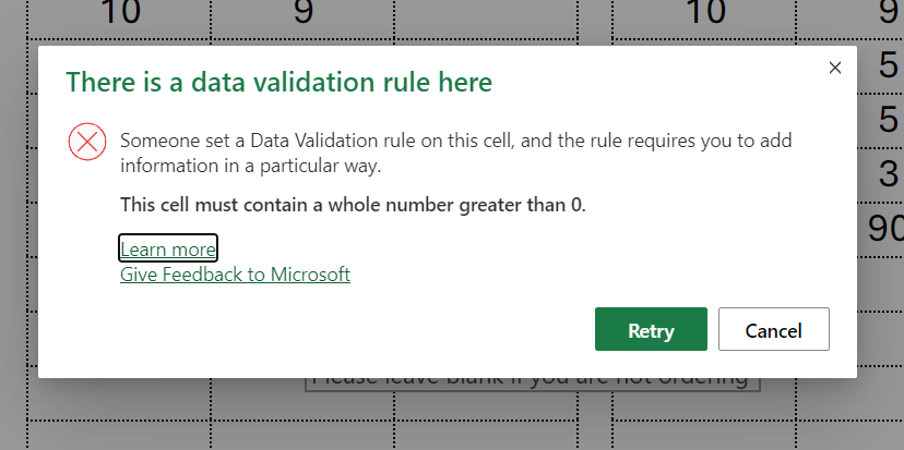 data validation warning
We can improve upon this by setting a custom message here too, though. And we can select whether to block it outright or to allow a zero to be entered after the warning pops up. Effectively allowing the warning to be ignored in the event that there's a reason to do this.
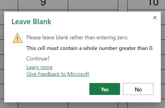 data validation custom warning message
And finally, we can couple any of these options with our conditional formatting so that if we do only warn against the entry, we still blot it out with the white text and white fill color.
The accompanying Excel Sheet and Google Sheet contain four columns of each of the above examples for you to see in action.
I hope this has been helpful for you!
Please come see my video tutorials on YouTube. I'd appreciate a like and subscribe as I'm growing my tech education channel there!
Have a great one!