By Sachin Malhotra
Do you know the amount of global air traffic in 2017? Do you know what the rise has been for air traffic over the past several years ? Well, lets look at some statistics.
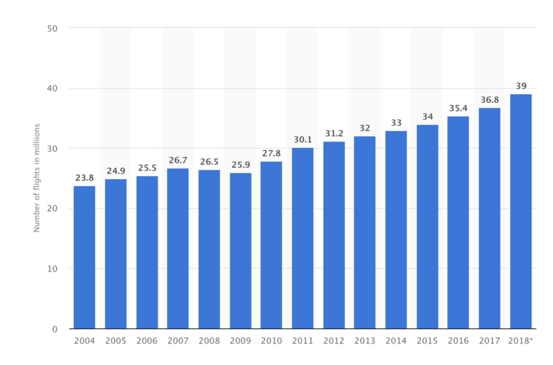
According to the International Civil Aviation Organization (ICAO), a record 4.1 billion passengers were carried by the aviation industry on scheduled services in 2017. And, the number of flights rose to 37 million globally in 2017.
That’s a lot of passengers and a lot of flights occupying the air space on a daily basis across the world. Since there are hundreds and thousands of these flights all around the globe, there are bound to be different routes with multiple stops in between from one place to another.
Every flight has a source and destination of its own and a standard economy seat price associated with it. Let’s leave out the fancy business class tickets and extra leg room and what not!
In such a scenario, it is too confusing to choose what flight would be the best one if we want to go from one place to another.
Let’s see the number of flight options StudentUniverse (provides discounts for students ?) gives me from Los Angeles to New Delhi.
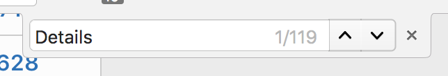
119 total flights are being offered. Then there appears a pop up on the website saying that there are other websites that might be offering similar flights at even cheaper rates. ?
So many websites and uncountable flights for just a single source and destination.
As a developer, if I want to solve this problem, I would build a system to efficiently address the following queries:
- Total number of destinations reachable (with a max number of stops) from my current location, and also list those destinations.
One should keep their options open when they want to travel ?. - It is a known fact (IMO ?) that a route with multiple stops tends to be a cheaper alternative to direct flights.
So, given a source and a destination, we may want to find routes with at least 2 or 3 stops. - Most importantly: What is the cheapest route from a given source to a given destination?
- And…. We’ll come to this one in the end ?.
As you might guess, there would be potentially thousands of flights as the output of the first two queries. But we can certainly reduce that by providing some other criteria to lessen the output size. For the scope of this article, let us focus on these original queries themselves.
Modeling the Flight Network as a Graph
It’s pretty clear from the headline of this article that graphs would be involved somewhere, isn’t it?
Modeling this problem as a graph traversal problem greatly simplifies it and makes the problem much more tractable. So, as a first step, let us define our graph.
We model the air traffic as a:
- directed
- possibly cyclic
- weighted
- forest. G (V, E)
Directed because every flight will have a designated source and a destination. These carry a lot of meaning.
Cyclic because it is very possible to follow a bunch of flights starting from a given location and ending back at the same location.
Weighted because every flight has a cost associated with it which would be the economy class flight ticket for this article.
And finally, a forest because we might have multiple connected components. It is not necessary that all the cities in the world have some sort of flight network between them. So, the graph can be disconnected, and hence a forest.
The vertices, V, would be the locations all over the world wherever there are working airports.
The edges, E, would be representative of all the flights constituting the air traffic. An edge from u -->; v simply means you have a directed flight from the location / node u to v .
Now that we have an idea about how to model the flight network as a graph, let us move on and solve the first common query that a user might have.
Total Number of Destinations Reachable
Who doesn’t like to travel?
As someone who likes to explore different places, you would want to know what all destinations are reachable from your local airport. Again, there would be additional criteria here to reduce the results of this query. But to keep things simple, we will simply try and find all the locations reachable from our local airport.
Now that we have a well defined graph, we can apply traversal algorithms to process it.
Starting off from a given point, we can use either Breadth First Search (BFS) or Depth First Search (DFS) to explore the graph or the locations reachable from the starting location within a maximum number of stops. Since this article is all about the breadth first search algorithm, let’s look at how we can use the famous BFS to accomplish this task.
We will initialize the BFS queue with the given location as the starting point. We then perform the breadth first traversal, and keep going until the queue is empty or until the maximum number of stops have been exhausted.
Note: If you are not familiar with the breadth first search or depth first search, I would recommend going through this article before continuing.
Let’s look at the code to initialize our graph data structure. We also need to look at how the BFS algorithm would end up giving us all the destinations reachable from a given source.
Now that we have a good idea about how the graph is to be initialized, let’s look at the code for the BFS algorithm.
Performing bfs on the city of Los Angeles would give us the following destinations which are reachable:
{'Chicago', 'France', 'Ireland', 'Italy', 'Japan', 'New Delhi', 'Norway'}
That was simple, wasn’t it?
We will look at how we can limit the BFS to a maximum number of stops later on in the article.
In case we have a humongous flight network, which we would have in a production scenario, then we would not ideally want to explore all the reachable destinations from a given starting point.
This is a use case if the flight network is very small or pertains only to a few regions in the United States.
But, for a large network, a more realistic use case would be to find all the flight routes with multiple stops. Let us look at this problem in some more detail and see how we can solve it.
Routes with multiple stops
It is a well known fact that more often than not, for a given source and destination, a multi stop trip is cheaper than a direct, non-stop flight.
A lot of times we prefer the direct flight to avoid the layovers. Also because the multi-stop flights do tend to take a lot of time — which we don’t have.
However, if you don’t have any deadlines approaching and you want to save some bucks (and are comfortable with the multi-stop route that a lot of airlines suggest), then you might actually benefit a lot from something like this.
Also, you might get to pass through some of the most beautiful locations in the world with some of the most advanced airports which you can enjoy. So, that’s enough motivation as it is.
In terms of the graph model that we have been talking about, given a source and a destination, we need to come up with routes with 2 or more stops for a given source and destination.
As an end user, we might not want to see flights in this order for this query:
[A, C, D, B], 2 stops, $X[A, E, D, C, F, W, G, T, B], 8 stops, $M[A, R, E, G, B], 3 stops, $K[A, Z, X, C, V, B, N, S, D, F, G, H, B, 11 stops, $P
I know. Nobody in their right minds would want to go for a flight route with 11 stops. But the point I’m trying to make is that an end user would want symmetry. Meaning that they would want to see all the flights with 2 stops first, then all the flights with 3 stops and so on till maybe a max of, say, 5 stops.
But, all the flight routes with the same number of stops in between should be displayed together. That is a requirement we need to satisfy.
Let’s look at how we can solve this. So, given the graph of flight networks, a source S and a destination D, we have to perform a level order traversal and report flight routes from S -->; D with at least 2 and at most 5 stops in between. This means we have to do a level order traversal until a depth of 7 from the start node S .
Have a look at the code for solving this problem:
This might not be the best way to go about solving this problem at scale — the largest memory constraint would be due to the nodes currently present in the queue.
Since every node or location can have thousands of flights to other destinations in the world, the queue could be humongous if we store actual flight data like this. This is just to demonstrate one of the use cases of the breadth first search algorithm.
Now, let us just focus on the traversal and look at the way it is done. The traversal algorithm is simple as it is. However, the entire space complexity of the level order traversal comes from the elements in the queue and the size of each element.
There are multiple ways to implement the algorithm. Also, each of them varies in terms of maximum memory consumed at any given time by the elements in the queue.
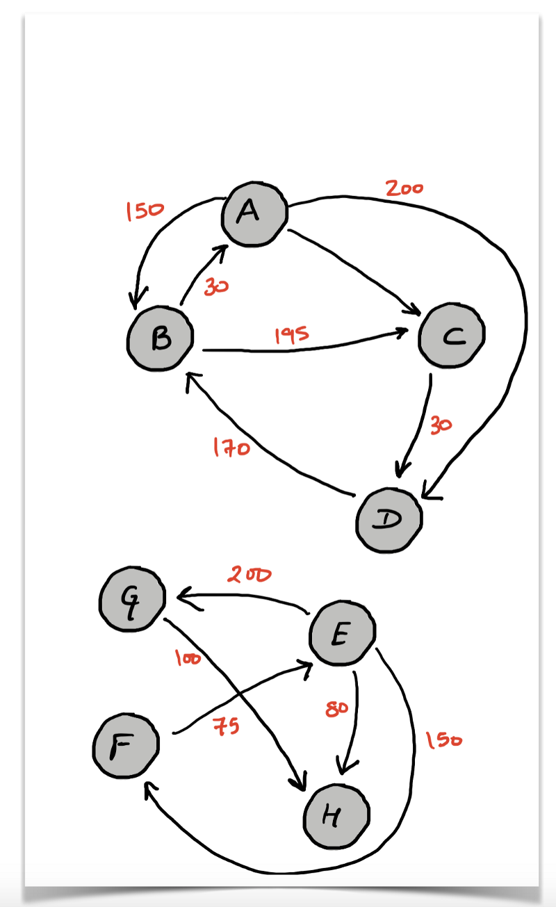
We want to see the maximum memory consumed by the queue at any point in time during the level order traversal. Before that, let’s construct a random flight network with random prices.
Now let us look at the implementation of level order traversal.
This above is the easiest and most straightforward implementation of the level order traversal algorithm.
With every node we add to the queue, we also store the level information and we push a tuple of (node, level) into the queue. So every time we pop an element from the queue, we have the level information attached with the node itself.
The level information for our use case would mean the number of stops from the source to this location in the flight route.
It turns out that we can do better as far as memory consumption of the program is concerned. Let us look at a slightly better approach to doing level order traversal.
The idea here is that we don’t store any additional information with the nodes being pushed into the queue. We use a None object to mark the end of a given level. We don’t know the size of any level before hand except for the first level, which just has our source node.
So, we start the queue with [source, None] and we keep popping elements. Every time we encounter a None element, we know that a level has ended and a new one has started. We push another None to mark the end of this new level.
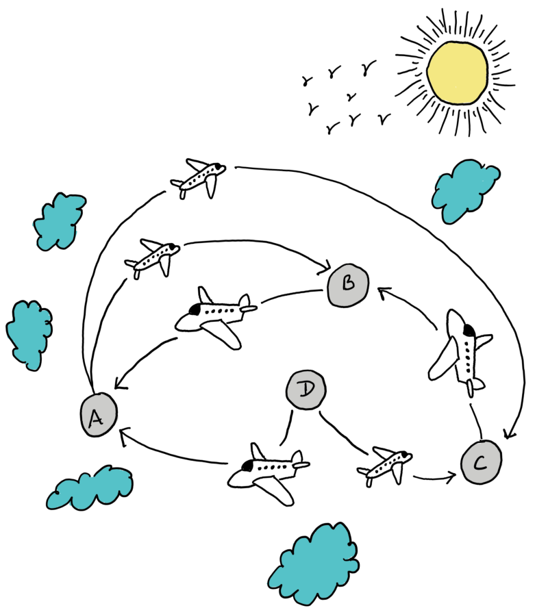
Consider a very simple graph here, and then we will dry run this through the graph.

**************************************************** LEVEL 0 beginslevel = 0, queue = [A, None]level = 0, pop, A, push, B, C, queue = [None, B, C]pop None ******************************************* LEVEL 1 beginspush Nonelevel = 1, queue = [B, C, None]level = 1, pop, B, push, C, D, F, queue = [C, None, C, D, F]level = 1, pop, C, push, D, D (lol!), queue = [None, C, D, F, D, D]pop None ******************************************* LEVEL 2 beginspush Nonelevel = 2, queue = [C, D, F, D, D, None] .... and so on
I hope this sums up the algorithm pretty well. This certainly is a neat trick to do level order traversal, keep track of the levels, and not encounter too much of a memory concern. This certainly reduces the memory footprint of the code.
Don’t get complacent now thinking this is a great improvement.
It is, but you should be asking two questions:
- How big of an improvement is this?
- Can we do better?
I will answer both of these questions now starting with the second question. The answer to that is Yes!
We can do one better here and completely do away with the need for the None in the queue. The motivation for this approach comes from the previous approach itself.
If you look closely at the dry run above, you can see that every time we pop a None, one level is finished and the other one is ready for processing. The important thing is that an entire next level exists in the queue at the time of popping of a None . We can make use of this idea of considering the queue size into the traversal logic.
Here is the pseudo code for this improved algorithm:
queue = Queue()queue.push(S)level = 0while queue is not empty { size = queue.size() // size represents the number of elements in the current level for i in 1..size { element = queue.pop() // Process element here // Perform a series of queue.push() operations here
level += 1
And here is the code for the same.
The pseudo code is self explanatory. We essentially do away with the need for an extra None element per level and instead make use of the queue’s size to change levels. This would also lead to improvement over the last method, but how much?
Have a look at the following Jupyter Notebook to see the memory difference between the three methods.
- We track the maximum size of the queue at any time by considering the sum of sizes of individual queue elements.
- According to Python’s documentation,
sys.getsizeofreturns the object’s pointer or reference’s size in bytes. So, we saved almost 4.4Kb space(20224 — 15800 bytes)by switching to theNonemethod from the original level order traversal method. This is just the memory savings for this random example, and we went only until the 5th level in the traversal. - The final method only gives an improvement of 16 bytes over the
Nonemethod. This is because we got rid of just 4Noneobjects which were being used to mark the 4 levels (apart from the first one) that we processed. Each pointer’s size (pointer to an object) is 4 bytes in Python on a 32 bit system.
Now that we have all these interesting multi-path routes from our source to our destination and highly efficient level order traversal algorithms to solve it, we can look at a more lucrative problem to solve using our very own BFS.
What’s the cheapest flight route from my source to a given destination? This is something everybody would be instantly interested in. I mean who doesn’t want to save some bucks?
Shortest Path from a given source to destination
There’s not much description to give for the problem statement. We just need to find the shortest path and make the end user happy.
Algorithmically, given a weighted directed graph, we need to find the shortest path from source to destination. Shortest or cheapest would be one and the same thing from the point of the view of the algorithm.
We will not go into describing a possible BFS solution to this problem because such a solution would be intractable. Let us look at the graph below to understand why that is the case.
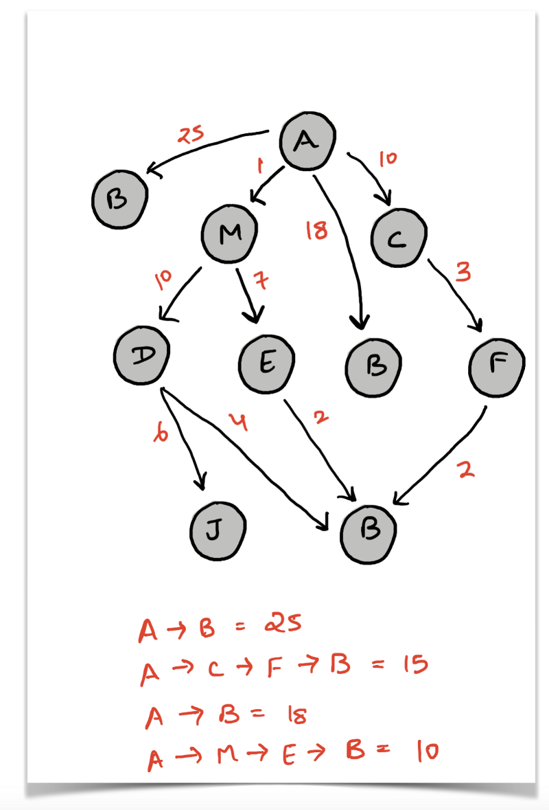
We say that BFS is the algorithm to use if we want to find the shortest path in an undirected, unweighted graph. The claim for BFS is that the first time a node is discovered during the traversal, that distance from the source would give us the shortest path.
The same cannot be said for a weighted graph. Consider the graph above. If say we were to find the shortest path from the node A to B in the undirected version of the graph, then the shortest path would be the direct link between A and B. So, the shortest path would be of length 1 and BFS would correctly find this for us.
However, we are dealing with a weighted graph here. So, the first discovery of a node during traversal does not guarantee the shortest path for that node. For example, in the diagram above, the node B would be discovered initially because it is the neighbor of A and the cost associated with this path (an edge in this case) would be 25 . But, this is not the shortest path. The shortest path is A --> M --> E --> B of length 10.
Breadth first search has no way of knowing if a particular discovery of a node would give us the shortest path to that node. And so, the only possible way for BFS (or DFS) to find the shortest path in a weighted graph is to search the entire graph and keep recording the minimum distance from source to the destination vertex.
This solution is not feasible for a huge network like our flight network that would have potentially thousands of nodes.
We won’t go into the details of how we can solve this. That is out of scope for this article.
What if I told you that BFS is just the right algorithm to find the shortest path in a weighted graph with a slight constraint ?
Constrained Shortest Paths
Since the graph we would have for the flight network is humongous, we know that exploring it completely is not really a possibility.
Consider the problem of shortest paths from the customer’s perspective. When you want to book a flight, these are the following options you ideally consider:
- It shouldn’t be too long a flight.
- It should be under your budget (Very Important).
- It may have multiple stops but not more than
KwhereKcan vary from person to person. - Finally we have personal preferences which involve things like lounge access, food quality, layover locations, and average leg room.
The important point to consider here is the third one above: it may have multiple stops, but not more than K where K can vary from person to person.
A customer wants the cheapest flight route, but they also don’t want say 20 stops in between their source and destination. A customer might be okay with a maximum of 3 stops, or in extreme cases maybe even 4 — but not more than that.
We would want an application that would find out the cheapest flight route with at most K stops for a given source and destination.
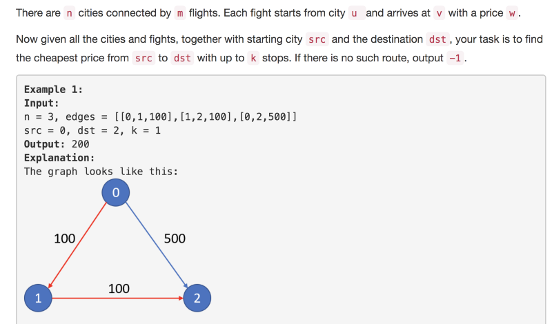
This question from LeetCode has been the primary motivation for me to write this article. I strongly recommend going through the question once and not only relying on the snapshot above.
“Why would BFS work here?” one might ask. “This is also a weighted graph and the same reason for the failure of BFS that we discussed in the previous section should apply here.” NO!
The number of levels that the search would go to is limited by the value K in the question or in the description provided at the start of section. So, essentially, we would be trying to find the shortest path, but we won’t have to explore the entire graph as such. We will just go up to the level K.
From a real life scenario, the value of K would be under 5 for any sane traveler ?.
Let us look at the pseudo-code for the algorithm:
def bfs(source, destination, K): min_cost = dictionary representing min cost under K stops for each node reachable from source.
set min_cost of source to be 0
Q = queue() Q.push(source) stops = 0 while Q is not empty {
size = Q.size for i in range 1..size { element = Q.pop()
if element == destination then continue
for neighbor in adjacency list of element { if stops == K and neighbor != destination then continue
if min_cost of neighbor improves, update and add back to the queue. } } stops ++ }
This again is level order traversal and the approach being used here is the one that makes use of the queue’s size at every level. Let us look at a commented version of the code to solve this problem.
Essentially, we keep track of the minimum distance of every node from the given source. The minimum distance for the source would be 0 and +inf for all others initially.
Whenever we encounter a node, we check if the current minimum path length can be improved or not. If it can be improved, that means that we have found an alternate path from source to this vertex with cheaper cost — a cheaper flight route until this vertex. We queue this vertex again so that locations and nodes reachable from this vertex on are updated (may or may not be) as well.
The key thing is this:
# No need to update the minimum cost if we have already exhausted our K stops. if stops == K and neighbor != dst: continue
So we just popped the a node represented by element in the code and neighbor can either be a destination or a random other node. If we have already exhausted our K stops with the element being the Kth stop, then we shouldn’t process and update (possibly) the minimum distance for neighbor. This would violate our maximum K stops condition in that case.
As it turns out, I solved this problem originally using Dynamic Programming and it took around 165ms to run on the LeetCode platform. I ran using BFS and it was blazing fast with just 45ms to execute. Motivation enough to write this article for you guys.
I hope you were able to derive some benefit from this article on Breadth First Search and some of its applications. The major focus was to showcase its application to shortest paths in a weighted graph under some constraints ?.