by Jerin Paul

How I developed a C.N.N. that recognizes emotions and broke into the Kaggle top 10

A baby starts to recognize its parents’ faces when it is just a couple of weeks old. As it grows, this innate ability improves. By the time it is a few months old, it starts to display social cues and is able to understand basic emotions like a smile.

Thanks to millions of years of evolution, we are able to understand each other without using a single word. Just a look and that is all that takes to understand whether a person is crestfallen or elated. Well, I tried teaching computers to do just that. This article is a detailed account of how the whole experiment turned out. Follow along as we recreate the network.

Cut to the chase Paul, please, give me the code. Don’t want fancy reading? No problem. You can find the code for this project here.

A Brief Introduction

“The best and most beautiful things in the world cannot be seen or even touched. They must be felt with the heart” ― Helen Keller

Hellen Keller excellently described the essence of human emotions in the aforementioned quote. What was once reserved for animals is no longer limited to them. Machine learning is catching on at a mindnumbing pace. The onset of convolutional neural networks was a breakthrough and changed the way computers “look” at the world.

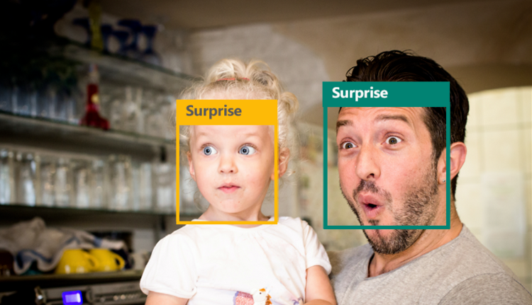
Facial expressions are nothing more than the arrangement of facial muscles to convey a certain emotional state to the observer. Emotions can be divided into six broad categories — Anger, Disgust, Fear, Happiness, Sadness, Surprise, and Neutral. In this M.L. project, we will train a model to differentiate between these.

We will train a convolutional neural network using the FER2013 dataset and will use various hyper-parameters to fine-tune the model. We will train it on Google Colab, which is a research project created to disseminate ML education. They will allocate you some resources like G.P.U. or T.P.U., and these can be used to train your model faster. The best part is that it is completely free.

Peek at the data

We will start by uploading the FER2013.csv file to our drive so that we can access it from Google Colab. There are 35,888 images in this dataset which are classified into six emotions. The data file contains 3 columns — Class, Image data, and Usage.

Class: is a digit between 0 to 6 and represents the emotion depicted in the corresponding picture. Each emotion is mapped to an integer as shown below.

0 - 'Angry'1 - 'Disgust'2 - 'Fear' 3 - 'Happy' 4 - 'Sad' 5 - 'Surprise'6 - 'Neutral'

Image data: is a string of 2,304 numbers and these are the pixel intensity values of our image, we will cover this in detail in a while.

Usage: denotes whether the corresponding data should be used to train the network or test it.

Decomposing an image.

As we all know that images are composed of pixels and these pixels are nothing more than numbers. Colored images have three color channels — red, green, and blue — and each channel is represented by a grid (2-dimensional array). Each cell in the grid stores a number between 0 and 255 which denotes the intensity of that cell.

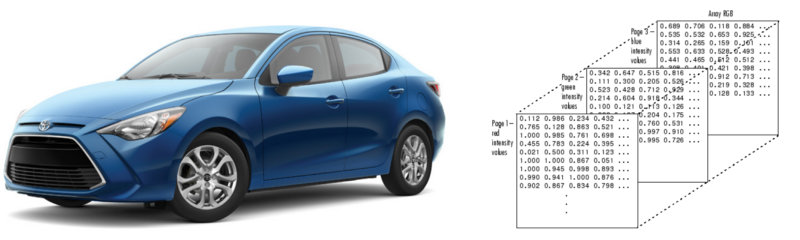
When these three channels are aligned together we get the images that we see.

Importing Necessary Libraries

%matplotlib inlineimport matplotlib.pyplot as plt

import numpy as npfrom keras.utils import to_categoricalfrom sklearn.model_selection import train_test_split

from keras.models import Sequential #Initialise our neural network model as a sequential networkfrom keras.layers import Conv2D #Convolution operationfrom keras.layers.normalization import BatchNormalizationfrom keras.regularizers import l2from keras.layers import Activation#Applies activation functionfrom keras.layers import Dropout#Prevents overfitting by randomly converting few outputs to zerofrom keras.layers import MaxPooling2D # Maxpooling functionfrom keras.layers import Flatten # Converting 2D arrays into a 1D linear vectorfrom keras.layers import Dense # Regular fully connected neural networkfrom keras import optimizersfrom keras.callbacks import ReduceLROnPlateau, EarlyStopping, TensorBoard, ModelCheckpointfrom sklearn.metrics import accuracy_score

Define Data Loading Mechanism

Now, we will define the load_data() function which will efficiently parse the data file and extract necessary data and then convert it into a usable image format.

All the images in our dataset are 48x48 in dimension. Since these images are gray-scale, there is only one channel. We will extract the image data and rearrange it into a 48x48 array. Then convert it into unsigned integers and divide it by 255 to normalize the data. 255 is the maximum possible value of a single cell. By dividing every element by 255, we ensure that all our values range between 0 and 1.

We will check the Usage column and store the data in separate lists, one for training the network and the other for testing it.

def load_data(dataset_path):

data = []  test_data = []  test_labels = []  labels =[]

  with open(dataset_path, 'r') as file:      for line_no, line in enumerate(file.readlines()):          if 0 < line_no <= 35887:            curr_class, line, set_type = line.split(',')            image_data = np.asarray([int(x) for x in line.split()]).reshape(48, 48)            image_data =image_data.astype(np.uint8)/255.0                        if (set_type.strip() == 'PrivateTest'):                            test_data.append(image_data)              test_labels.append(curr_class)            else:              data.append(image_data)              labels.append(curr_class)            test_data = np.expand_dims(test_data, -1)      test_labels = to_categorical(test_labels, num_classes = 7)      data = np.expand_dims(data, -1)         labels = to_categorical(labels, num_classes = 7)          return np.array(data), np.array(labels), np.array(test_data), np.array(test_labels)

Once our data is segregated, we will expand the dimensions of both testing and training data by one to accommodate the channel. Then, we will one hot encode all the labels using the to_categorical() function and return all the lists as numpy arrays.

We will load the data by calling the load_data() function.

dataset_path = "/content/gdrive/My Drive/Colab Notebooks/Emotion Recognition/Data/fer2013.csv"

train_data, train_labels, test_data, test_labels = load_data(dataset_path)

print("Number of images in Training set:", len(train_data))print("Number of images in Test set:", len(test_data))

Our data is loaded and now let us get to the best part, defining the network.

Defining the model.

We will use Keras to create a Sequential Convolutional Network. Which means that our neural network will be a linear stack of layers. This network will have the following components:

1. Convolutional Layers: These layers are the building blocks of our network and these compute dot product between their weights and the small regions to which they are linked. This is how these layers learn certain features from these images.
2. Activation functions: are those functions which are applied to the outputs of all layers in the network. In this project, we will resort to the use of two functions— Relu and Softmax.
3. Pooling Layers: These layers will downsample the operation along the dimensions. This helps reduce the spatial data and minimize the processing power that is required.
4. Dense layers: These layers are present at the end of a C.N.N. They take in all the feature data generated by the convolution layers and do the decision making.
5. Dropout Layers: randomly turns off a few neurons in the network to prevent overfitting.
6. Batch Normalization: normalizes the output of a previous activation layer by subtracting the batch mean and dividing by the batch standard deviation. This speeds up the training process.

model.add(Conv2D(64, (3, 3), activation='relu', input_shape=(48, 48, 1), kernel_regularizer=l2(0.01)))model.add(Conv2D(64, (3, 3), padding='same',activation='relu'))model.add(BatchNormalization())model.add(MaxPooling2D(pool_size=(2,2), strides=(2, 2)))model.add(Dropout(0.5))    model.add(Conv2D(128, (3, 3), padding='same', activation='relu'))model.add(BatchNormalization())model.add(Conv2D(128, (3, 3), padding='same', activation='relu'))model.add(BatchNormalization())model.add(Conv2D(128, (3, 3), padding='same', activation='relu'))model.add(BatchNormalization())model.add(MaxPooling2D(pool_size=(2,2)))model.add(Dropout(0.5))    model.add(Conv2D(256, (3, 3), padding='same', activation='relu'))model.add(BatchNormalization())model.add(Conv2D(256, (3, 3), padding='same', activation='relu'))model.add(BatchNormalization())model.add(Conv2D(256, (3, 3), padding='same', activation='relu'))model.add(BatchNormalization())model.add(MaxPooling2D(pool_size=(2,2)))model.add(Dropout(0.5))    model.add(Conv2D(512, (3, 3), padding='same', activation='relu'))model.add(BatchNormalization())model.add(Conv2D(512, (3, 3), padding='same', activation='relu'))model.add(BatchNormalization())model.add(Conv2D(512, (3, 3), padding='same', activation='relu'))model.add(BatchNormalization())model.add(MaxPooling2D(pool_size=(2,2)))model.add(Dropout(0.5))    model.add(Flatten())model.add(Dense(512, activation='relu'))model.add(Dropout(0.5))model.add(Dense(256, activation='relu'))model.add(Dropout(0.5))model.add(Dense(128, activation='relu'))model.add(Dropout(0.5))model.add(Dense(64, activation='relu'))model.add(Dropout(0.5))model.add(Dense(7, activation='softmax'))

We will compile the network using Adam optimizer and will use a variable learning rate. Since we are dealing with a classification problem that involves multiple categories, we will use categorical_crossentropy as our loss function.

adam = optimizers.Adam(lr = learning_rate)

model.compile(optimizer = adam, loss = 'categorical_crossentropy', metrics = ['accuracy'])    print(model.summary()

Callback functions

Callback functions are those functions which are called after every epoch during the training process. We will be using the following callback functions:

1. ReduceLROnPlateau: Training a neural network can plateau at times and we stop seeing any progress during this stage. Therefore, this function monitors the validation loss for signs of a plateau and then alter the learning rate by the specified factor if a plateau is detected.

lr_reducer = ReduceLROnPlateau(monitor='val_loss', factor=0.9, patience=3)

2. EarlyStopping: At times, the progress stalls while training a neural network and we stop seeing any improvement in the validation accuracy (in this case). Majority of the time, this means that the network won’t converge any further and there is no point in continuing the training process. This function waits for a specified number of epochs and terminates the training if no change in the parameter is found.

early_stopper = EarlyStopping(monitor='val_acc', min_delta=0, patience=6, mode='auto')

3. ModelCheckpoint: Training neural networks generally takes a lot of time and anything can happen during this period that may result in loss of all the variables and weights. Creating checkpoints is a good habit as it saves your model after every epoch. In case your training stops you can load the checkpoint and resume the process.

checkpointer = ModelCheckpoint('/content/gdrive/My Drive/Colab Notebooks/Emotion Recognition/Model/weights.hd5', monitor='val_loss', verbose=1, save_best_only=True)

Time to train

All our hard work is about to be put to the test. But before we fit the model, let us define some hyper-parameters.

epochs = 100batch_size = 64learning_rate = 0.001

Our data will pass through the model 100 times and in batches of 64 images. We will use 20% of our training data to validate the model after every epoch.

model.fit(          train_data,          train_labels,          epochs = epochs,          batch_size = batch_size,          validation_split = 0.2,          shuffle = True,          callbacks=[lr_reducer, checkpointer, early_stopper]          )

Now that the network is being trained, I suggest that you go and finish that book you started or go for a run. It took me about an hour on Google Colab.

Test the model

Remember the private set we stored separately? That was for this very moment. This is the moment of truth and this is where we will reap the fruit of our labor.

predicted_test_labels = np.argmax(model.predict(test_data), axis=1)test_labels = np.argmax(test_labels, axis=1)print ("Accuracy score = ", accuracy_score(test_labels, predicted_test_labels))

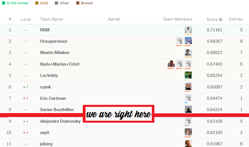
Well, the results came back and we scored 63.167%. On first glance, it isn’t much but we broke into the ninth position of the Facial Emotion Recognition Kaggle competition.

Now, pat yourself on the back and start brainstorming about the ways in which you can improve this model. We can use better hyper-parameters or create a different network architecture altogether to achieve higher accuracies.

Save the model

Quickly save the model using model_from_json from keras.models.

from keras.models import model_from_json

model_json = model.to_json()with open("/content/gdrive/My Drive/Colab Notebooks/Emotion Recognition/FERmodel.json", "w") as json_file:    json_file.write(model_json)# serialize weights to HDF5model.save_weights("/content/gdrive/My Drive/Colab Notebooks/Emotion Recognition/FERmodel.h5")print("Saved model to disk")

Wrapping it all up

We started off by defining a loading mechanism and loading the images. Then we created a training set and a testing set. Then we defined a fine model and defined a few callback functions. We went over the basic components of a convolutional neural network and then we trained our network.

I extended this project by creating a python application which is able to detect faces and recognize their emotions in real time. That will be covered in a later post.

We just accomplished something that was part of science fiction a few decades ago. Yet there is a lot left to learn. The internet provides us with a plethora of information to constantly create and learn. May the learning never cease.