By Ljubica Lazarevic
If you're curious about graph databases and how they compare with relational database management systems, then this beginner-friendly guide is for you.
In this article, you'll discover of the power of graphs by working with a small movie data set. It is based on the built in dataset and guide available on the Neo4j Sandbox.
Want to drive right in and have a go yourself? Please do! You’ll find instructions on how to get up and running here.

What We'll Cover in This Article
Graph databases are growing in popularity and adoption. With ever-larger amounts of data from many different sources, it's critical to be able to understand the data and see how it's all connected.
If you want to find out more about the kinds of problems graph databases help solve, and how you might spot a good application for one, here's an introductory blog post.
Some of you reading on may have heard of graph databases (GDB), some you perhaps haven’t. In this article we’re going to cover exactly what they are, and how they compare to the more traditional, Relational Database Management Systems (RDBMS) which have been the stalwart software application of the past 40+ years.
Inspired by a small movie data set used by Neo4j as a guided introduction to graph querying, we are going to look at side-by-side examples and equivalents of what a data model or query would look like in both a graph database, and a relational database.
In this article, we will:
- Introduce graph databases, briefly covering the two models that exist
- Take a conceptual look at the differences between relational and graph paradigms
- Look at the movie data set, and compare and contrast data models from a GDB and a RDBMS perspective
- Compare and contrast some queries, based on either Cypher (for GDB) or SQL
- Talk through the more interesting queries that appear in the movie example, and break out exactly what is happening
If you’d like to have a play with the example walkthrough movie data set before reading the article (or during!), you are more than welcome to do so. You can find out more here.
What is a Graph Database?
First of all, before we dive into what a graph database is, let’s define the term. Graph databases are a type of “Not only SQL” (NoSQL) data store. They are designed to store and retrieve data in a graph structure.
The storage mechanism used can vary from database to database. Some GDBs may use more traditional database constructs, such as table-based, and then have a graph API layer on top.
Others will be ‘native’ GDBs – where the whole construct of the database from storage, management and query maintains the graph structure of the data. Many of the graph databases currently available do this by treating relationships between entities as first class citizens.
Different Types of Graph Databases
There are broadly two types of GDB, Resource Descriptive Framework (RDF)/triple stores/semantic graph databases, and property graph databases.
An RDF GDB uses the concept of a triple, which is a statement composed of three elements: subject-predicate-object.
Subject will be a resource or nodes in the graph, object will be another node or literal value, and predicate represents the relationship between subject and object. There are no internal structures on the nodes or relationships, and everything is identified by a unique identifier, in the form of a URI.
The motivation behind this structure is exchanging and publishing data. To find out more about this structure, I would refer you to Jesus Barrasa’s work in this space.
A Property GDB is focussed on the concept of storing data that is close to the logical model. This in turn will be based on the questions sought of the data itself, and focuses on making that representation as efficient as possible for storage and querying.
Unlike an RDF-based graph, there are internal structures on the nodes and relationships, lending to a rich representation of data as well as associated metadata.
The following two diagrams provide a side by side comparison of sample data represented in a Property Graph Database, and as an RDF graph – both of which representing the person Tom Hanks, acting the role Jim Lovell, in the movie Apollo 13.


Anatomy of a Property Graph Database
For the rest of this article, we will be focussing on native property graph databases, specifically Neo4j. Let's check out the main components.
The main components of a property graph database are as follows:
- Node: also known as a vertex in graph theory – the main data element from which graphs are constructed
- Relationship: also known as an edge in graph theory – a link between two nodes. It will have direction and a type. A node without relationships is permitted, a relationship without two nodes is not permitted
 Node and Relationship
- Label: Defines a node category, a node can have more than one
- Property: Enriches a node or relationship, no need for nulls!
 Label, Type, and Property
Graph Databases vs Relational Databases
Relational Databases Recap
A lot of developers are familiar with the traditional relational database, where data is stored in tables within a well-defined schema.
Each row in the table is a discrete entity of data. One of these elements in the row is typically used to define its uniqueness: the primary key. It could be a unique ID or maybe something like a social security number for a person.
We then go through a process called normalization to reduce data repetition. In normalization, we’re moving references, something like an address for a person, into another table. So we get a reference from the row representing the entity to the row representing the address for that person.
If, for example, somebody changes their address, you wouldn’t want multiple versions of that person’s addresses everywhere and have to try and remember all the different instances of where that person’s addresses exist. Normalization makes sure you have one version of the data, so you can make the updates in one place.
Then when we query, we want to reconstitute this normalized data. We do what’s called a JOIN operation.
In our main entity row, we have the primary key that identifies the ID for the entity, let’s say the person. We also have what’s called a foreign key that represents a row in our address table. We join the two tables through their primary and foreign keys, and use that to look up the address in the address table. This is called a JOIN and these JOINs are done at query time and at read time.
When we’re doing a JOIN in a relational database, it’s a set comparison operation where we’re looking to see where our two sets of data overlap (in this case, the sets are the person table and the address table). At a high level, that’s how traditional relational databases work.


How Native Graph Databases Work: Connections and Index-Free Adjacency
Let’s have a quick peek at a native graph database and how it works.
We spoke about the discrete entity in a relational database being a row within a table. In a native graph database, that row would be the equivalent of a node. It’s still a discrete entity, so we still have this element of normalization.
A node would be an entity. If we were having person nodes, we would have one node for one person. And we would have some degree of uniqueness in it, let’s say the social security number.
The key difference, however, is when we are connecting this person node to another discrete entity – for example, an address – we create a physical connection (aka relationship) between those two points.
The address would have a pointer that says, what is the outbound part of the relationship that connects to the node? We then have another pointer for the inbound part of the relationship pointing to the other node.
So, effectively, we’re collecting a set of pointers, and this is a manifestation of the physical connection between those two entities. That is the big difference.
In a relational database, you would reconstitute the data with joins on read, which means at query time, it would go off to try and figure out how things map together.
In a graph database, since we already know these two elements are connected, we don’t need to look up the mapping at query time. All we’re doing is following the stored relationships to the other nodes.
This is something we call index-free adjacency. This concept of index-free adjacency is key to understanding the performance optimizations of a native graph database compared to other database systems.
Index-free adjacency means that during a local graph traversal, following these pointers (relationships) that connect the nodes in my graph, the performance of the operation is not dependent on the overall size of the graph. It depends on the number of relationships connected to the nodes that you’re traversing.
When we talk of a JOIN being a set operation (intersection), we’re using an index in a relational database to see where those two sets overlap. This means that the performance of the JOIN operation starts to slow down as the tables get bigger.
In big O notation terms, this is something like logarithmic growth using an index — something like O(log n) and also grows exponentially with the number of JOINs in your query.
On the other hand, traversing relationships in the graph is more of linear growth based on the number of relationships in the nodes that we’re actually traversing, not the overall size of the graph.
This is the fundamental query time optimization that graph databases make that give us index-free adjacency. From a performance perspective, that is really the most important thing to think about when we think of a native graph database.
A Brief Introduction to the Movie Graph
We've spoken a fair bit about the theoretical differences between a graph and relational database. Now let's start to look at some side-by-side comparisons.
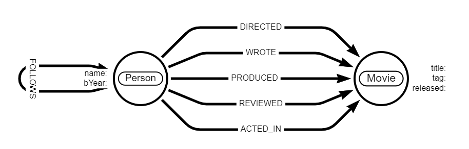
The movie graph consists of a data set consisting of actors, directors, producers, writers, reviewers and movies, along with information on how they all connect to each other.
This data set is available within Neo4j Browser, and can be easily triggered by using the :PLAY movies command. As a reminder, here's a blog to show you how to get started.
The Movies data set consists of:
- 133 Person nodes/entities
- 38 Movie nodes/entities
- 253 relationships/connections between the above entities, describing connections such as:
- Person(s) who directed a Movie
- Person(s) who acted in a Movie and role(s) played
- Person(s) who wrote a Movie
- Person(s) who produced a Movie
- Person(s) who have reviewed a Movie and score and summary given
- Person(s) who follow another Person
While it is a relatively small data set, it comprehensively describes the power of graphs.
Comparing data models
First of all, let's take a look at the data models of our respective databases. As with all data models, what they look like will ultimately depend on the types of questions you are asking. So let's assume we're going to ask the following types of questions:
- What movies did a person act in?
- What movies does a person have a connection with?
- Who are all the co-actors a person has ever worked with?
Based on these, here are the associated potential data models:
 Entity Relationship data model for movie graph
 Property Graph data model for movie graph
Immediately you will spot something – those IDs have gone! As we are connecting data together as soon as we know there's a connection there, we no longer need them, or those mapping tables to let us know how different rows of data connect together.
Comparing queries
Let's now move on to comparing some queries. Taking a few of the first queries from the :PLAY movies example, let's look at some side-by-side comparisons of the Cypher query, and what would the equivalent SQL query look like.
What is Cypher, I hear you ask? Cypher is a graph query language which is used to query the Neo4j graph database. There is an OpenCypher version too, which is used by a number of other vendors.
As we move through the queries, it should start to become clearer how a graph database, accompanied with a query language to help explore relationships really starts to come into its own. Let's start looking for Tom Hanks!
How to find Tom Hanks
MATCH (p:Person {name: "Tom Hanks"})
RETURN p
SELECT * FROM person
WHERE person.name = "Tom Hanks"
How to find Tom Hanks movies
MATCH (:Person {name: “Tom Hanks”})-->(m:Movie)
RETURN m.title
SELECT movie.title FROM movie
INNER JOIN movie_person ON movie.movie_id = person_movie.movie_id
INNER JOIN person ON person_movie.person_id = person.person_id
WHERE person.name = "Tom Hanks"
How to find movies Tom Hanks has directed
MATCH (:Person {name: "Tom Hanks"})-[:DIRECTED]->(m:Movie)
RETURN m.title
SELECT movie.title FROM movie
INNER JOIN person_movie ON movie.movie_id = person_movie.movie_id
INNER JOIN person ON person_movie.person_id = person.person_id
INNER JOIN involvement ON person_movie.involve_id = involvement.involve_id
WHERE person.name = "Tom Hanks" AND involvement.title = "Director"
How to find co-actors of Tom Hanks
MATCH (:Person {name: "Tom Hanks"})-->(:Movie)<-[:ACTED_IN]-(coActor:Person)
RETURN coActor.name
WITH tom_movies AS (
    SELECT movie.movie_id FROM movie
    INNER JOIN person_movie ON movie.movie_id = person_movie.movie_id
    INNER JOIN person ON person_movie.person_id = person.person_id
    WHERE person.name = "Tom Hanks")
SELECT person.name FROM person
INNER JOIN person_movie ON tom_movies = person_movie.movie_id
INNER JOIN person ON person_movie.person_id = person.person_id
INNER JOIN involvement ON person_movie.involve_id = involvement.involve_id
WHERE involvement.title = "Actor"
More Queries with Cypher
Hopefully you’ll get the idea of the differences between Cypher and SQL queries. Perhaps you’re excited to learn more about them too! We’ll have some references further on in the blog post.
For now, let’s have a look at some of the other Cypher queries you can find in the :PLAY movies graph example, and explain what’s going on.
No movie graph would be complete without the quintessential Bacon number question, and our movie graph is no different!
Up until now, the examples we have looked at have always traversed one relationship each time. We can easily take advantage of those ‘joins on write’ to traverse many relationships to answer interesting questions.
So, back to the Kevin Bacon number. The following query will start at the Kevin Bacon person node, and then go up to 4 hops out from that start point, to bring back all connected movies and people.
MATCH (bacon:Person {name:"Kevin Bacon"})-[*1..4]-(hollywood)
RETURN DISTINCT hollywood
We can do this by using the syntax of *1..4 in the relationship part of the query pattern:
*indicates everything1..4indicates the range - 1 says from 1 hop away, 4 says up to 4 hops away
Another graphy thing we could do on this movie data set is the shortest path between two nodes.
In this example, let’s find out the shortest path between Kevin Bacon and Meg Ryan. You will spot we’re using the * syntax again for the relationship pattern – indicating everything.
What may be new to you is the p=. You’ve seen how we use references for nodes (e.g. bacon or meg in our current query), and we can do the same for relationships.
We can also have references for the whole path (that is, all the nodes and relationships involved). The syntax we use for that is refName =, which in this example is p=.
We also use the Cypher function shortestPath() – this is a simple shortest path function that will return the first shortest path between two specified nodes. Be aware there may be another, equally short path, but this simple function will just bring back the first one encountered.
For those of you interested in other path-related functions, check out the ones available in APOC and GDS.
MATCH p=shortestPath(
(bacon:Person {name:"Kevin Bacon"})-[*]-(meg:Person {name:"Meg Ryan"}))
RETURN p
A word of warning to you all: you may see that [*] and be tempted to run your graph without the constraint of the shortestPath() function or the 1..4 range. But this may well result in something unexpected.
In our example with Kevin Bacon and Meg Ryan, even though there are only 253 relationships in this very small data set, all of the possible combinations of paths between nodes and relationships could easily run into millions of different paths between Bacon and Ryan.
When using * in your relationships as part of a query, use with extreme caution! This problem does not come up with shortest path because as a potential path that is longer than the currently identified shortest one is encountered, it is immediately dropped.
A simple recommendations query
Here are two queries that really show the power of graph databases and we can easily use the connections in our data to make some recommendations.
In our first query we’re looking for new co-actors for Tom Hanks to work with who he’s not already worked with. The query does this by:
- Firstly, finding all of the co-actors he has already worked with
- Then, finding all of the co-actors' co-actors (referred to as co-co-actors)
- Next, we want to exclude those co-co-actors who have already worked with Tom, as well as making sure the co-co-actor isn’t Tom himself
- Finally, we return the suggested co-co-actors names, and we’re going to order them but the number of co-actors that have worked with them – the more co-actors that have worked with that co-co-actor, the better the recommendation.
MATCH (tom:Person {name:"Tom Hanks"})-[:ACTED_IN]->(m)<-[:ACTED_IN]-(coActors),
(coActors)-[:ACTED_IN]->(m2)<-[:ACTED_IN]-(cocoActors)
WHERE NOT (tom)-[:ACTED_IN]->()<-[:ACTED_IN]-(cocoActors)
    AND tom <> cocoActors
RETURN cocoActors.name AS Recommended, count(*) AS Strength
    ORDER BY Strength DESC
Excellent, so we’ve found some potential co-co-actors. In this next query, we want to suggest Tom Cruise as a potential new co-actor for Tom Hanks to work with. But, who’s going to introduce these Toms to each other? Back to the movie graph we go.
In this query, we:
- Find the co-actors of Tom Hanks, and then find which out of those co-actors have also acted with Tom Cruise
- Then we’ll return the co-actor and the movies they were in with both Tom Hanks and Tom Cruise
MATCH (tom:Person {name:"Tom Hanks"})-[:ACTED_IN]->(m)<-[:ACTED_IN]-(coActors),
(coActors)-[:ACTED_IN]->(m2)<-[:ACTED_IN]-(cruise:Person {name:"Tom Cruise"})
RETURN tom, m, coActors, m2, cruise
Last Words
We've come to the end of our walk through of the movies database example. Hopefully those of you with a relational database background have a better idea of the similarities and differences between relational and graph databases, as well as a taste of the Cypher query language.
If you're keen to learn more about modeling and querying Neo4j, do check out the free Graph Academy.