By Bipin Krishnan P
In this article, we'll be going under the hood of neural networks to learn how to build one from the ground up.
The one thing that excites me the most in deep learning is tinkering with code to build something from scratch. It's not an easy task, though, and teaching someone else how to do so is even more difficult.
I've been working my way through the Fast.ai course and this blog is greatly inspired by my experience.
Without any further delay let's start our wonderful journey of demystifying neural networks.
How does a neural network work?
Let's start by understanding the high level workings of neural networks.
A neural network takes in a data set and outputs a prediction. It's as simple as that.
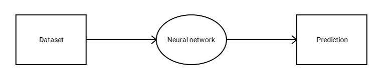 How a neural network works
Let me give you an example.
Let's say that one of your friends (who is not a great football fan) points at an old picture of a famous footballer – say Lionel Messi – and asks you about him.
You will be able to identify the footballer in a second. The reason is that you have seen his pictures a thousand times before. So you can identify him even if the picture is old or was taken in dim light.
But what happens if I show you a picture of a famous baseball player (and you have never seen a single baseball game before)? You will not be able to recognize that player. In that case, even if the picture is clear and bright, you won't know who it is.
This is the same principle used for neural networks. If our goal is to build a neural network to recognize cats and dogs, we just show the neural network a bunch of pictures of dogs and cats.
More specifically, we show the neural network pictures of dogs and then tell it that these are dogs. And then show it pictures of cats, and identify those as cats.
Once we train our neural network with images of cats and dogs, it can easily classify whether an image contains a cat or a dog. In short, it can recognize a cat from a dog.
But if you show our neural network a picture of a horse or an eagle, it will never identify it as horse or eagle. This is because it has never seen a picture of a horse or eagle before because we have never shown it those animals.
If you wish to improve the capability of the neural network, then all you have to do is show it pictures of all the animals that you want the neural network to classify. As of now, all it knows is cats and dogs and nothing else.
The data set we use for our training heavily depends on the problem on our hands. If you wish to classify whether a tweet has a positive or negative sentiment, then probably, you will want a data set containing a lot of tweets with their corresponding label as either positive or negative.
Now that you have a high-level overview of data sets and how a neural network learns from that data, let's dive deeper into how neural networks work.
Understanding neural networks
We will be building a neural network to classify the digits three and seven from an image.
But before we build our neural network, we need to go deeper to understand how they work.
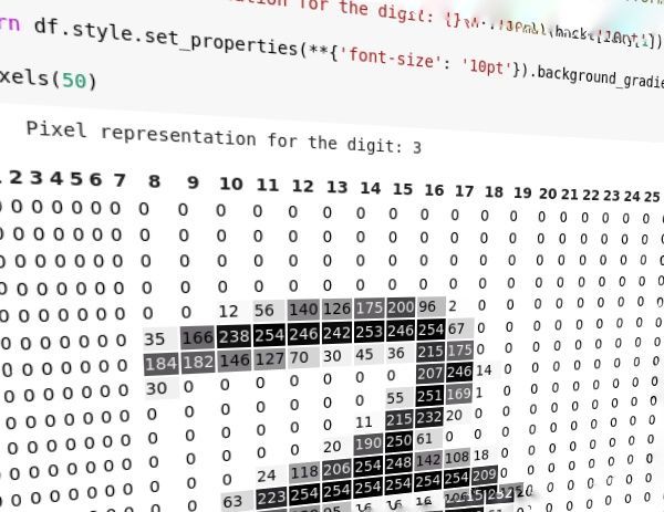
Every image that we pass to our neural network is just a bunch of numbers. That is, each of our images has a size of 28×28 which means it has 28 rows and 28 columns, just like a matrix.
We see each of the digits as a complete image, but to a neural network, it is just a bunch of numbers ranging from 0 to 255.
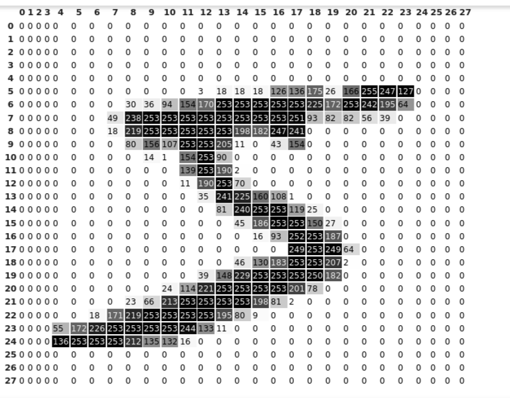
Here is a pixel representation of the digit five:
 Pixel values along with shades
As you can see above, we have 28 rows and 28 columns (the index starts from 0 and ends at 27) just like a matrix. Neural networks only see these 28×28 matrices.
To show some more details, I've just shown the shade along with the pixel values. If you look closer into the image, you can see that the pixel values close to 255 are darker whereas the values closer to 0 are lighter in shade.
In PyTorch we don't use the term matrix. Instead, we use the term tensor. Every number in PyTorch is represented as a tensor. So, from now on, we will use the term tensor instead of matrix.
Visualizing a neural network
A neural network can have any number of neurons and layers.
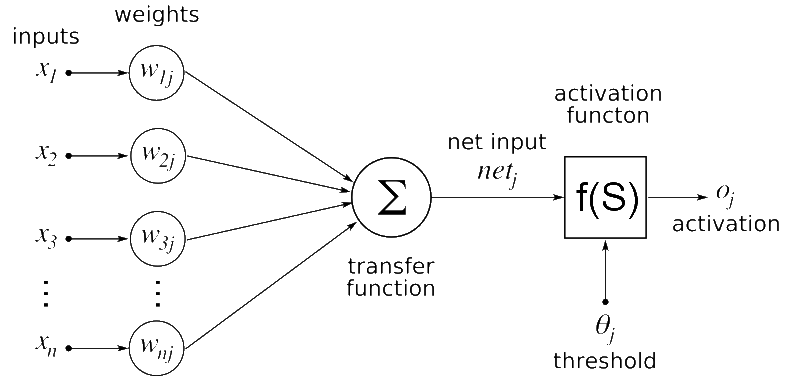
This is how a neural network looks:
 Artificial neural network
Don't get confused by the Greek letters in the picture. I will break it down for you:
Take the case of predicting whether a patient will survive or not based on a data set containing the name of the patient, temperature, blood pressure, heart condition, monthly salary, and age.
In our data set, only the temperature, blood pressure, heart condition, and age have significant importance for predicting whether the patient will survive or not. So we will assign a higher weight value to these values in order to show higher importance.
But features like the name of the patient and monthly salary have little or no influence on the patient's survival rate. So we assign smaller weight values to these features to show less importance.
In the above figure, x1, x2, x3...xn are the features in our data set which may be pixel values in the case of image data or features like blood pressure or heart condition as in the above example.
The feature values are multiplied by the corresponding weight values referred to as w1j, w2j, w3j...wnj. The multiplied values are summed together and passed to the next layer.
The optimum weight values are learned during the training of the neural network. The weight values are updated continuously in such a way as to maximize the number of correct predictions.
The activation function is nothing but the sigmoid function in our case. Any value we pass to the sigmoid gets converted to a value between 0 and 1. We just put the sigmoid function on top of our neural network prediction to get a value between 0 and 1.
You will understand the importance of the sigmoid layer once we start building our neural network model.
There are a lot of other activation functions that are even simpler to learn than sigmoid.
This is the equation for a sigmoid function:
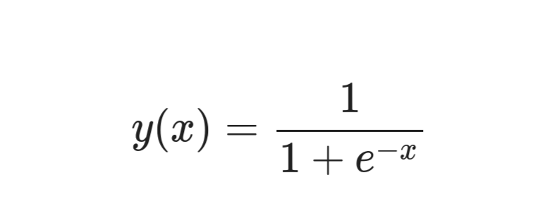 Sigmoid function
The circular-shaped nodes in the diagram are called neurons. At each layer of the neural network, the weights are multiplied with the input data.
We can increase the depth of the neural network by increasing the number of layers. We can improve the capacity of a layer by increasing the number of neurons in that layer.
Understanding our data set
The first thing we need in order to train our neural network is the data set.
Since the goal of our neural network is to classify whether an image contains the number three or seven, we need to train our neural network with images of threes and sevens. So, let's build our data set.
Luckily, we don't have to create the data set from scratch. Our data set is already present in PyTorch. All we have to do is just download it and do some basic operations on it.
We need to download a data set called MNIST (Modified National Institute of Standards and Technology) from the torchvision library of PyTorch.
Now let's dig deeper into our data set.
What is the MNIST data set?
The MNIST data set contains handwritten digits from zero to nine with their corresponding labels as shown below:
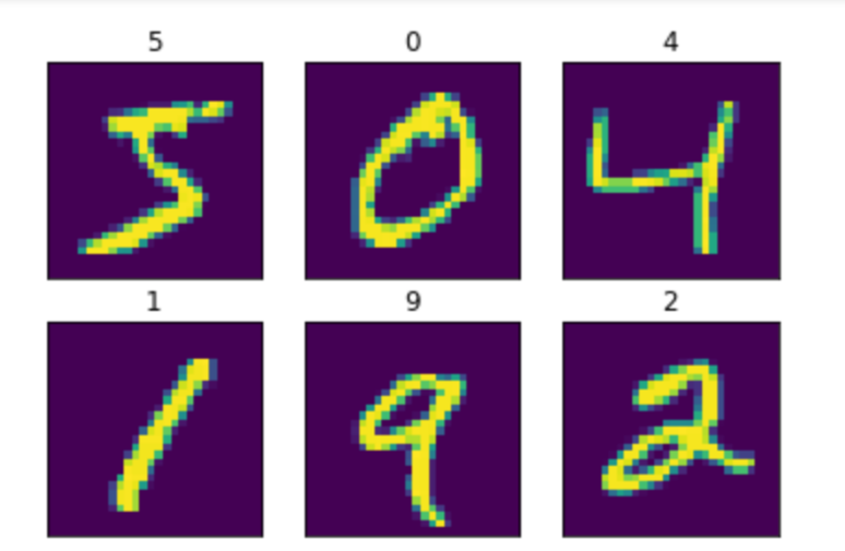 MNIST data set
So, what we do is simply feed the neural network the images of the digits and their corresponding labels which tell the neural network that this is a three or seven.
How to prepare our data set
The downloaded MNIST data set has images and their corresponding labels.
We just write the code to index out only the images with a label of three or seven. Thus, we get a data set of threes and sevens.
First, let's import all the necessary libraries.
import torch
from torchvision import datasets
import matplotlib.pyplot as plt
We import the PyTorch library for building our neural network and the torchvision library for downloading the MNIST data set, as discussed before. The Matplotlib library is used for displaying images from our data set.
Now, let's prepare our data set.
mnist = datasets.MNIST('./data', download=True)

threes = mnist.data[(mnist.targets == 3)]/255.0
sevens = mnist.data[(mnist.targets == 7)]/255.0

len(threes), len(sevens)
As we learned above, everything in PyTorch is represented as tensors. So our data set is also in the form of tensors.
We download the data set in the first line. We index out only the images whose target value is equal to 3 or 7 and normalize them by dividing with 255 and store them separately.
We can check whether our indexing was done properly by running the code in the last line which gives the number of images in the threes and sevens tensor.
Now let's check whether we've prepared our data set correctly.
def show_image(img):
  plt.imshow(img)
  plt.xticks([])
  plt.yticks([])
  plt.show()

show_image(threes[3])
show_image(sevens[8])
Using the Matplotlib library, we create a function to display the images.
Let's do a quick sanity check by printing the shape of our tensors.
print(threes.shape, sevens.shape)
If everything went right, you will get the size of threes and sevens as ([6131, 28, 28]) and ([6265, 28, 28]) respectively. This means that we have 6131 28×28 sized images for threes and 6265 28×28 sized images for sevens.
We've created two tensors with images of threes and sevens. Now we need to combine them into a single data set to feed into our neural network.
combined_data = torch.cat([threes, sevens])
combined_data.shape
We will concatenate the two tensors using PyTorch and check the shape of the combined data set.
Now we will flatten the images in the data set.
flat_imgs = combined_data.view((-1, 28*28))
flat_imgs.shape
We will flatten the images in such a way that each of the 28×28 sized images becomes a single row with 784 columns (28×28=784). Thus the shape gets converted to ([12396, 784]).
We need to create labels corresponding to the images in the combined data set.
target = torch.tensor([1]*len(threes)+[2]*len(sevens))
target.shape
We assign the label 1 for images containing a three, and the label 0 for images containing a seven.
How to train your Neural Network
To train your neural network, follow these steps.
Step 1: Building the model
Below you can see the simplest equation that shows how neural networks work:
y = Wx + b
Here, the term 'y' refers to our prediction, that is, three or seven. 'W' refers to our weight values, 'x' refers to our input image, and 'b' is the bias (which, along with weights, help in making predictions).
In short, we multiply each pixel value with the weight values and add them to the bias value.
The weights and bias value decide the importance of each pixel value while making predictions.
We are classifying three and seven, so we have only two classes to predict.
So, we can predict 1 if the image is three and 0 if the image is seven. The prediction we get from that step may be any real number, but we need to make our model (neural network) predict a value between 0 and 1.
This allows us to create a threshold of 0.5. That is, if the predicted value is less than 0.5 then it is a seven. Otherwise it is a three.
We use a sigmoid function to get a value between 0 and 1.
We will create a function for sigmoid using the same equation shown earlier. Then we pass in the values from the neural network into the sigmoid.
We will create a single layer neural network.
We cannot create a lot of loops to multiply each weight value with each pixel in the image, as it is very expensive. So we can use a magic trick to do the whole multiplication in one go by using matrix multiplication.
def sigmoid(x): return 1/(1+torch.exp(-x))

def simple_nn(data, weights, bias): return sigmoid((data@weights) + bias)
Step 2: Defining the loss
Now, we need a loss function to calculate by how much our predicted value is different from that of the ground truth.
For example, if the predicted value is 0.3 but the ground truth is 1, then our loss is very high. So our model will try to reduce this loss by updating the weights and bias so that our predictions become close to the ground truth.
We will be using mean squared error to check the loss value. Mean squared error finds the mean of the square of the difference between the predicted value and the ground truth.
def error(pred, target): return ((pred-target)**2).mean()
Step 3: Initialize the weight values
We just randomly initialize the weights and bias. Later, we will see how these values are updated to get the best predictions.
w = torch.randn((flat_imgs.shape[1], 1), requires_grad=True)
b = torch.randn((1, 1), requires_grad=True)
The shape of the weight values should be in the following form:
(Number of neurons in the previous layer, number of neurons in the next layer)
We use a method called gradient descent to update our weights and bias to make the maximum number of correct predictions.
Our goal is to optimize or decrease our loss, so the best method is to calculate gradients.
We need to take the derivative of each and every weight and bias with respect to the loss function. Then we have to subtract this value from our weights and bias.
In this way, our weights and bias values are updated in such a way that our model makes a good prediction.
Updating a parameter for optimizing a function is not a new thing – you can optimize any arbitrary function using gradients.
We've set a special parameter (called requires_grad) to true to calculate the gradient of weights and bias.
Step 4: Update the weights
If our prediction does not come close to the ground truth, that means that we've made an incorrect prediction. This means that our weights are not correct. So we need to update our weights until we get good predictions.
For this purpose, we put all of the above steps inside a for loop and allow it to iterate any number of times we wish.
At each iteration, the loss is calculated and the weights and biases are updated to get a better prediction on the next iteration.
Thus our model becomes better after each iteration by finding the optimal weight value suitable for our task in hand.
Each task requires a different set of weight values, so we can't expect our neural network trained for classifying animals to perform well on musical instrument classification.
This is how our model training looks like:
for i in range(2000):
  pred = simple_nn(flat_imgs, w, b)
  loss = error(pred, target.unsqueeze(1))
  loss.backward()

  w.data -= 0.001*w.grad.data
  b.data -= 0.001*b.grad.data

  w.grad.zero_()
  b.grad.zero_()

print("Loss: ", loss.item())
We will calculate the predictions and store it in the 'pred' variable by calling the function that we've created earlier. Then we calculate the mean squared error loss.
Then, we will calculate all the gradients for our weights and bias and update the value using those gradients.
We've multiplied the gradients by 0.001, and this is called learning rate. This value decides the rate at which our model will learn, if it is too low, then the model will learn slowly, or in other words, the loss will be reduced slowly.
If the learning rate is too high, our model will not be stable, jumping between a wide range of loss values. This means it will fail to converge.
We do the above steps for 2000 times, and each time our model tries to reduce the loss by updating the weights and bias values.
We should zero out the gradients at the end of each loop or epoch so that there is no accumulation of unwanted gradients in the memory which will affect our model's learning.
Since our model is very small, it doesn't take much time to train for 2000 epochs or iterations. After 2000 epochs, our neural netwok has given a loss value of 0.6805 which is not bad from such a small model.
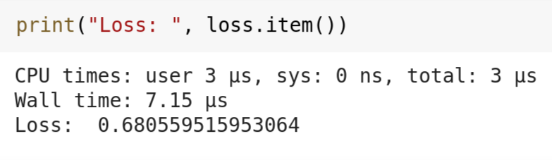 Final result
Conclusion
There is a huge space for improvement in the model that we've just created.
This is just a simple model, and you can experiment on it by increasing the number of layers, number of neurons in each layer, or increasing the number of epochs.
In short, machine learning is a whole lot of magic using math. Always learn the foundational concepts – they may be boring, but eventually you will understand that those boring math concepts created these cutting edge technologies like deepfakes.
You can get the complete code on GitHub or play with the code in Google colab.