by Anne Bonner

How to build an image classifier with greater than 97% accuracy

A clear and complete blueprint for success

How do you teach a computer to look at an image and correctly identify it as a flower? How do you teach a computer to see an image of a flower and then tell you exactly what species of flower it is when even you don’t know what species it is?

Let me show you!

This article will take you through the basics of creating an image classifier with PyTorch. You can imagine using something like this in a phone app that tells you the name of the flower your camera is looking at. You could, if you wanted, train this classifier and then export it for use in an application of your own.

What you do from here depends entirely on you and your imagination.

I put this article together for anyone out there who’s brand new to all of this and looking for a place to begin. It’s up to you to take this information, improve on it, and make it your own!

If you want to view the notebook, you can find it here.

Because this PyTorch image classifier was built as a final project for a Udacity program, the code draws on code from Udacity which, in turn, draws on the official PyTorch documentation. Udacity also provided a JSON file for label mapping. That file can be found in this GitHub repo.

Information about the flower data set can be found here. The data set includes a separate folder for each of the 102 flower classes. Each flower is labeled as a number and each of the numbered directories holds a number of .jpg files.

Let’s get started!

Because this is a neural network using a larger dataset than my CPU could handle in any reasonable amount of time, I went ahead and set up my image classifier in Google Colab. Colab is truly awesome because it provides free GPU. (If you’re new to Colab, check out this article on getting started with Google Colab!)

Because I was using Colab, I needed to start by importing PyTorch. You don’t need to do this if you aren’t using Colab.

*** UPDATE! (01/29)*** Colab now supports native PyTorch!!! You shouldn’t need to run the code below, but I’m leaving it up just in case anyone is having any issues!

# Import PyTorch if using Google Colab# http://pytorch.org/from os.path import existsfrom wheel.pep425tags import get_abbr_impl, get_impl_ver, get_abi_tagplatform = '{}{}-{}'.format(get_abbr_impl(), get_impl_ver(), get_abi_tag())cuda_output = !ldconfig -p|grep cudart.so|sed -e 's/.*\.\([0-9]*\)\.\([0-9]*\)$/cu\1\2/'accelerator = cuda_output[0] if exists('/dev/nvidia0') else 'cpu'

!pip install -q http://download.pytorch.org/whl/{accelerator}/torch-0.4.1-{platform}-linux_x86_64.whl torchvisionimport torch

Then, after having some trouble with Pillow (it’s buggy in Colab!), I just went ahead and ran this:

import PILprint(PIL.PILLOW_VERSION)

If you get anything below 5.3.0, use the dropdown menu under “Runtime” to “Restart runtime” and run this cell again. You should be good to go!

You’ll want to be using GPU for this project, which is incredibly simple to set up on Colab. You just go to the “runtime” dropdown menu, select “change runtime type” and then select “GPU” in the hardware accelerator drop-down menu!

Then I like to run

train_on_gpu = torch.cuda.is_available()

if not train_on_gpu:    print('Bummer!  Training on CPU ...')else:    print('You are good to go!  Training on GPU ...')

just to make sure it’s working. Then run

device = torch.device("cuda:0" if torch.cuda.is_available() else "cpu")

to define the device.

After this, import the files. There are a ton of ways to do this, including mounting your Google Drive if you have your dataset stored there, which is actually really simple. Even though I didn’t wind up finding that to be the most useful solution, I’m including that below, just because it’s so easy and useful.

from google.colab import drivedrive.mount('/content/gdrive')

Then you’ll see a link, click on that, allow access, copy the code that pops up, paste it in the box, hit enter, and you’re good to go! If you don’t see your drive in the side box on the left, just hit “refresh” and it should show up.

(Run the cell, click the link, copy the code on the page, paste it in the box, hit enter, and you’ll see this when you’ve successfully mounted your drive):

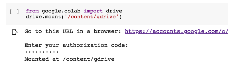
It’s actually super easy!

However, if you’d rather download a shared zip file link (this wound up being easier and faster for this project), you can use:

!wget !unzip

For example:

!wget -cq https://s3.amazonaws.com/content.udacity-data.com/courses/nd188/flower_data.zip!unzip -qq flower_data.zip

That will give you Udacity’s flower data set in seconds!

(If you’re uploading small files, you can just upload them directly with some simple code. However, if you want to, you can also just go to the left side of the screen and click “upload files” if you don’t feel like running some simple code to grab a local file.)

After loading the data, I imported the libraries I wanted to use:

%matplotlib inline%config InlineBackend.figure_format = 'retina'

import timeimport jsonimport copy

import matplotlib.pyplot as pltimport seaborn as snsimport numpy as npimport PIL

from PIL import Imagefrom collections import OrderedDict

import torchfrom torch import nn, optimfrom torch.optim import lr_schedulerfrom torch.autograd import Variableimport torchvisionfrom torchvision import datasets, models, transformsfrom torch.utils.data.sampler import SubsetRandomSamplerimport torch.nn as nnimport torch.nn.functional as F

Next comes the data transformations! You want to make sure to use several different types of transformations on your training set in order to help your program learn as much as it can. You can create a more robust model by training it on flipped, rotated, and cropped images.

The means that standard deviations are provided to normalize the image values before passing them to our network, but they can also be found by looking at the mean and standard deviation values of the different dimensions of the image tensors. The official documentation is incredibly helpful here!

For my image classifier, I kept it simple with:

data_transforms = {    'train': transforms.Compose([        transforms.RandomRotation(30),        transforms.RandomResizedCrop(224),        transforms.RandomHorizontalFlip(),        transforms.ToTensor(),        transforms.Normalize([0.485, 0.456, 0.406],                              [0.229, 0.224, 0.225])    ]),    'valid': transforms.Compose([        transforms.Resize(256),        transforms.CenterCrop(224),        transforms.ToTensor(),        transforms.Normalize([0.485, 0.456, 0.406],                              [0.229, 0.224, 0.225])    ])}

# Load the datasets with ImageFolderimage_datasets = {x: datasets.ImageFolder(os.path.join(data_dir, x),                                          data_transforms[x])                  for x in ['train', 'valid']}

# Using the image datasets and the trainforms, define the dataloadersbatch_size = 64dataloaders = {x: torch.utils.data.DataLoader(image_datasets[x], batch_size=batch_size,                                             shuffle=True, num_workers=4)              for x in ['train', 'valid']}

class_names = image_datasets['train'].classes

dataset_sizes = {x: len(image_datasets[x]) for x in ['train', 'valid']}class_names = image_datasets['train'].classes

As you can see above, I also defined the batch size, data loaders, and class names in the code above.

To take a very quick look at the data and check my device, I ran:

print(dataset_sizes)print(device)

{'train': 6552, 'valid': 818}cuda:0

Next, we need to do some mapping from the label number and the actual flower name. Udacity provided a JSON file for this mapping to be done simply.

with open('cat_to_name.json', 'r') as f:    cat_to_name = json.load(f)

In order to test the data loader, run:

images, labels = next(iter(dataloaders['train']))rand_idx = np.random.randint(len(images))# Print(rand_idx)print("label: {}, class: {}, name: {}".format(labels[rand_idx].item(),                                               class_names[labels[rand_idx].item()],                                               cat_to_name[class_names[labels[rand_idx].item()]]))

Now it starts to get even more exciting! A number of models in the last several years have been created by people far, far more qualified than most of us for reuse in computer vision problems. PyTorch makes it easy to load pre-trained models and build on them, which is exactly what we’re going to do for this project. The choice of model is entirely up to you!

Some of the most popular pre-trained models, like ResNet, AlexNet, and VGG, come from the ImageNet Challenge. These pre-trained models allow others to quickly obtain cutting-edge results in computer vision without needing such large amounts of computer power, patience, and time. I actually had great results with DenseNet and decided to use DenseNet161, which gave me very good results relatively quickly.

You can quickly set this up by running

model = models.densenet161(pretrained=True)

but it might be more interesting to give yourself a choice of model, optimizer, and scheduler. In order to set up a choice in architecture, run

model_name = 'densenet' #vggif model_name == 'densenet':    model = models.densenet161(pretrained=True)    num_in_features = 2208    print(model)elif model_name == 'vgg':    model = models.vgg19(pretrained=True)    num_in_features = 25088    print(model.classifier)else:    print("Unknown model, please choose 'densenet' or 'vgg'")

which allows you to quickly set up an alternate model.

After that, you can start to build your classifier, using the parameters that work best for you. I went ahead and built

for param in model.parameters():    param.requires_grad = False

def build_classifier(num_in_features, hidden_layers, num_out_features):       classifier = nn.Sequential()    if hidden_layers == None:        classifier.add_module('fc0', nn.Linear(num_in_features, 102))    else:        layer_sizes = zip(hidden_layers[:-1], hidden_layers[1:])        classifier.add_module('fc0', nn.Linear(num_in_features, hidden_layers[0]))        classifier.add_module('relu0', nn.ReLU())        classifier.add_module('drop0', nn.Dropout(.6))        classifier.add_module('relu1', nn.ReLU())        classifier.add_module('drop1', nn.Dropout(.5))        for i, (h1, h2) in enumerate(layer_sizes):            classifier.add_module('fc'+str(i+1), nn.Linear(h1, h2))            classifier.add_module('relu'+str(i+1), nn.ReLU())            classifier.add_module('drop'+str(i+1), nn.Dropout(.5))        classifier.add_module('output', nn.Linear(hidden_layers[-1], num_out_features))            return classifier

which allows for an easy way to change the number of hidden layers that I’m using, as well as quickly adjusting the dropout rate. You may decide to add additional ReLU and dropout layers in order to more finely hone your model.

Next, work on training your classifier parameters. I decided to make sure I only trained the classifier parameters here while having feature parameters frozen. You can get as creative as you want with your optimizer, criterion, and scheduler. The criterion is the method used to evaluate the model fit, the optimizer is the optimization method used to update the weights, and the scheduler provides different methods for adjusting the learning rate and step size used during optimization.

Try as many options and combinations as you can to see what gives you the best result. You can see all of the official documentation here. I recommend taking a look at it and making your own decisions about what you want to use. You don’t literally have an infinite number of options here, but it sure feels like it once you start playing around!

hidden_layers = None

classifier = build_classifier(num_in_features, hidden_layers, 102)print(classifier)

# Only train the classifier parameters, feature parameters are frozenif model_name == 'densenet':    model.classifier = classifier    criterion = nn.CrossEntropyLoss()    optimizer = optim.Adadelta(model.parameters())    sched = optim.lr_scheduler.StepLR(optimizer, step_size=4)elif model_name == 'vgg':    model.classifier = classifier    criterion = nn.NLLLoss()    optimizer = optim.Adam(model.classifier.parameters(), lr=0.0001)    sched = lr_scheduler.StepLR(optimizer, step_size=4, gamma=0.1)else:    pass

Now it’s time to train your model.

# Adapted from https://pytorch.org/tutorials/beginner/transfer_learning_tutorial.html

def train_model(model, criterion, optimizer, sched, num_epochs=5):    since = time.time()

best_model_wts = copy.deepcopy(model.state_dict())    best_acc = 0.0

for epoch in range(num_epochs):        print('Epoch {}/{}'.format(epoch+1, num_epochs))        print('-' * 10)

# Each epoch has a training and validation phase        for phase in ['train', 'valid']:            if phase == 'train':                model.train()  # Set model to training mode            else:                model.eval()   # Set model to evaluate mode

running_loss = 0.0            running_corrects = 0

# Iterate over data.            for inputs, labels in dataloaders[phase]:                inputs = inputs.to(device)                labels = labels.to(device)

# Zero the parameter gradients                optimizer.zero_grad()

# Forward                # track history if only in train                with torch.set_grad_enabled(phase == 'train'):                    outputs = model(inputs)                    _, preds = torch.max(outputs, 1)                    loss = criterion(outputs, labels)

# Backward + optimize only if in training phase                    if phase == 'train':                        #sched.step()                        loss.backward()                                                optimizer.step()

# Statistics                running_loss += loss.item() * inputs.size(0)                running_corrects += torch.sum(preds == labels.data)

epoch_loss = running_loss / dataset_sizes[phase]            epoch_acc = running_corrects.double() / dataset_sizes[phase]

print('{} Loss: {:.4f} Acc: {:.4f}'.format(                phase, epoch_loss, epoch_acc))

# Deep copy the model            if phase == 'valid' and epoch_acc > best_acc:                best_acc = epoch_acc                best_model_wts = copy.deepcopy(model.state_dict())

print()

time_elapsed = time.time() - since    print('Training complete in {:.0f}m {:.0f}s'.format(        time_elapsed // 60, time_elapsed % 60))    print('Best val Acc: {:4f}'.format(best_acc))

# Load best model weights    model.load_state_dict(best_model_wts)        return model

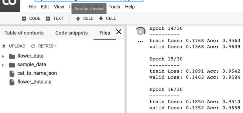
epochs = 30model.to(device)model = train_model(model, criterion, optimizer, sched, epochs)

I wanted to be able to monitor my epochs easily and also keep track of the time elapsed as my model was running. The code above includes both, and the results are pretty good! You can see that the model is quickly learning and the accuracy on the validation set quickly reached over 95% by epoch 7!

Epoch 1/30----------train Loss: 2.4793 Acc: 0.4791valid Loss: 0.9688 Acc: 0.8191Epoch 2/30----------train Loss: 0.8288 Acc: 0.8378valid Loss: 0.4714 Acc: 0.9010Epoch 3/30----------train Loss: 0.5191 Acc: 0.8890valid Loss: 0.3197 Acc: 0.9181Epoch 4/30----------train Loss: 0.4064 Acc: 0.9095valid Loss: 0.2975 Acc: 0.9169Epoch 5/30----------train Loss: 0.3401 Acc: 0.9214valid Loss: 0.2486 Acc: 0.9401Epoch 6/30----------train Loss: 0.3111 Acc: 0.9303valid Loss: 0.2153 Acc: 0.9487Epoch 7/30----------train Loss: 0.2987 Acc: 0.9298valid Loss: 0.1969 Acc: 0.9584

...

Training complete in 67m 43sBest val Acc: 0.973105

You can see that running this code on Google Colab with GPU took just over an hour.

Now it’s time for evaluation

model.eval()

accuracy = 0

for inputs, labels in dataloaders['valid']:    inputs, labels = inputs.to(device), labels.to(device)    outputs = model(inputs)        # Class with the highest probability is our predicted class    equality = (labels.data == outputs.max(1)[1])

# Accuracy = number of correct predictions divided by all predictions    accuracy += equality.type_as(torch.FloatTensor()).mean()    print("Test accuracy: {:.3f}".format(accuracy/len(dataloaders['valid'])))

Test accuracy: 0.973

It’s important to save your checkpoint

model.class_to_idx = image_datasets['train'].class_to_idx

checkpoint = {'input_size': 2208,              'output_size': 102,              'epochs': epochs,              'batch_size': 64,              'model': models.densenet161(pretrained=True),              'classifier': classifier,              'scheduler': sched,              'optimizer': optimizer.state_dict(),              'state_dict': model.state_dict(),              'class_to_idx': model.class_to_idx             }   torch.save(checkpoint, 'checkpoint.pth')

You don’t have to save all of the parameters, but I’m including them here as an example. This checkpoint specifically saves the model with a pre-trained densenet161 architecture, but if you want to save your checkpoint with the two-choice option, you can absolutely do that. Simply adjust the input size and model.

Now you’re able to load your checkpoint. If you’re submitting your project into the Udacity workspace, things can get a little tricky. Here’s some help with troubleshooting your checkpoint load.

You can check your keys by running

ckpt = torch.load('checkpoint.pth')ckpt.keys()

Then load and rebuild your model!

def load_checkpoint(filepath):    checkpoint = torch.load(filepath)    model = checkpoint['model']    model.classifier = checkpoint['classifier']    model.load_state_dict(checkpoint['state_dict'])    model.class_to_idx = checkpoint['class_to_idx']    optimizer = checkpoint['optimizer']    epochs = checkpoint['epochs']        for param in model.parameters():        param.requires_grad = False            return model, checkpoint['class_to_idx']

model, class_to_idx = load_checkpoint('checkpoint.pth')

Want to keep going? It’s a good idea to do some image preprocessing and inference for classification. Go ahead and define your image path and open an image:

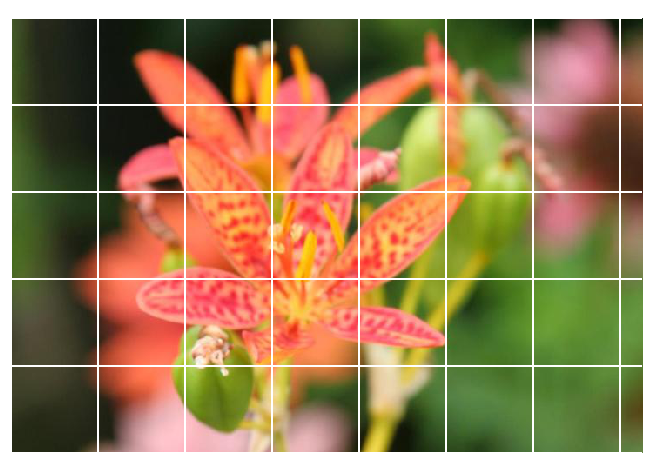
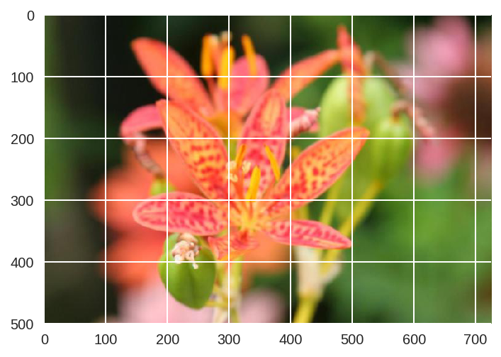
image_path = 'flower_data/valid/102/image_08006.jpg'img = Image.open(image_path)

Process your image and take a look at a processed image:

def process_image(image):    ''' Scales, crops, and normalizes a PIL image for a PyTorch model,        returns an Numpy array    '''    # Process a PIL image for use in a PyTorch model    # tensor.numpy().transpose(1, 2, 0)    preprocess = transforms.Compose([        transforms.Resize(256),        transforms.CenterCrop(224),        transforms.ToTensor(),        transforms.Normalize(mean=[0.485, 0.456, 0.406],                              std=[0.229, 0.224, 0.225])    ])    image = preprocess(image)    return image

def imshow(image, ax=None, title=None):    """Imshow for Tensor."""    if ax is None:        fig, ax = plt.subplots()        # PyTorch tensors assume the color channel is the first dimension    # but matplotlib assumes is the third dimension    image = image.numpy().transpose((1, 2, 0))        # Undo preprocessing    mean = np.array([0.485, 0.456, 0.406])    std = np.array([0.229, 0.224, 0.225])    image = std * image + mean        # Image needs to be clipped between 0 and 1 or it looks like noise when displayed    image = np.clip(image, 0, 1)        ax.imshow(image)        return ax

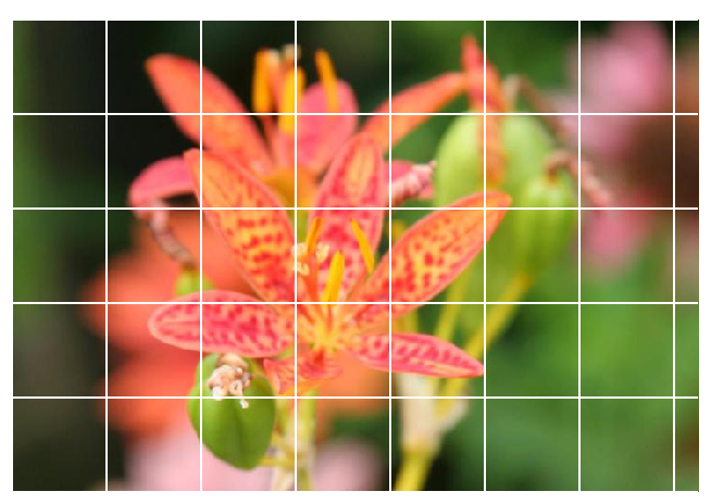
with Image.open('flower_data/valid/102/image_08006.jpg') as image:    plt.imshow(image)

model.class_to_idx = image_datasets['train'].class_to_idx

Create a function for prediction:

def predict2(image_path, model, topk=5):    ''' Predict the class (or classes) of an image using a trained deep learning model.    '''        # Implement the code to predict the class from an image file    img = Image.open(image_path)    img = process_image(img)        # Convert 2D image to 1D vector    img = np.expand_dims(img, 0)            img = torch.from_numpy(img)        model.eval()    inputs = Variable(img).to(device)    logits = model.forward(inputs)        ps = F.softmax(logits,dim=1)    topk = ps.cpu().topk(topk)        return (e.data.numpy().squeeze().tolist() for e in topk)

Once the images are in the correct format, you can write a function to make predictions with your model. One common practice is to predict the top 5 or so (usually called top-KK) most probable classes. You’ll want to calculate the class probabilities then find the KK largest values.

To get the top KK largest values in a tensor use k.topk(). This method returns both the highest k probabilities and the indices of those probabilities corresponding to the classes. You need to convert from these indices to the actual class labels using class_to_idx, which you added to the model or from the Image Folder you used to load the data. Make sure to invert the dictionary so you get a mapping from index to class as well.

This method should take a path to an image and a model checkpoint, then return the probabilities and classes.

img_path = 'flower_data/valid/18/image_04252.jpg'probs, classes = predict2(img_path, model.to(device))print(probs)print(classes)flower_names = [cat_to_name[class_names[e]] for e in classes]print(flower_names)

I was pretty pleased with how my model performed!

[0.9999195337295532, 1.4087702766119037e-05, 1.3897360986447893e-05, 1.1400215043977369e-05, 6.098791800468462e-06][12, 86, 7, 88, 40]['peruvian lily', 'desert-rose', 'king protea', 'magnolia', 'sword lily']

Basically, it’s nearly 100% likely that the image I specified is a Peruvian Lily. Want to take a look? Try using matplotlib to plot the probabilities for the top five classes in a bar graph along with the input image:

def view_classify(img_path, prob, classes, mapping):    ''' Function for viewing an image and it's predicted classes.    '''    image = Image.open(img_path)

fig, (ax1, ax2) = plt.subplots(figsize=(6,10), ncols=1, nrows=2)    flower_name = mapping[img_path.split('/')[-2]]    ax1.set_title(flower_name)    ax1.imshow(image)    ax1.axis('off')        y_pos = np.arange(len(prob))    ax2.barh(y_pos, prob, align='center')    ax2.set_yticks(y_pos)    ax2.set_yticklabels(flower_names)    ax2.invert_yaxis()  # labels read top-to-bottom    ax2.set_title('Class Probability')

view_classify(img_path, probs, classes, cat_to_name)

You should see something like this:

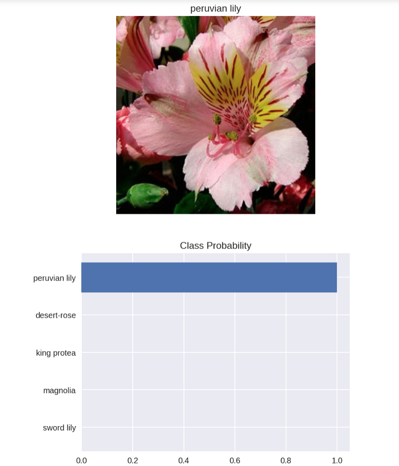
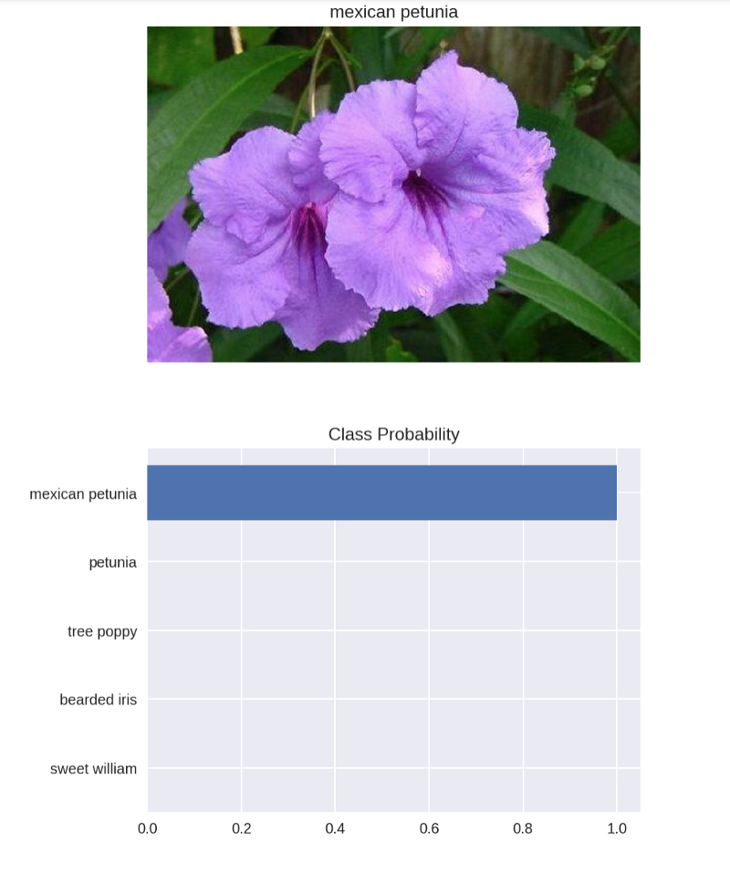
I’ve got to say, I’m pretty happy with that! I recommend testing a few other images to see how close your predictions are on a variety of images.

Now it’s time to make a model of your own and let me know how it goes in the responses below!

Have you finished your deep learning or machine learning model, but you don’t know what to do with it next? Why not deploy it to the internet?

Get your model out there so everyone can see it!

Check out this article to learn how to deploy your machine learning model with Flask!