By Aleksey Bilogur
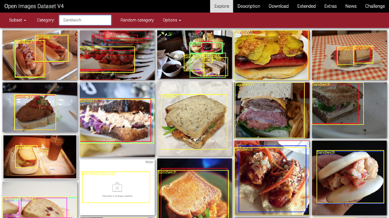
If you’re looking build an image classifier but need training data, look no further than Google Open Images.
This massive image dataset contains over 30 million images and 15 million bounding boxes. That’s 18 terabytes of image data!
Plus, Open Images is much more open and accessible than certain other image datasets at this scale. For example, ImageNet has restrictive licensing.
However, it’s not easy for developers on single machines to sift through that much data.You need to download and process multiple metadata files, and roll their own storage space (or apply for access to a Google Cloud bucket).
On the other hand, there aren’t many custom image training sets in the wild, because frankly they’re a pain to create and share.
In this article, we’ll build and distribute a simple end-to-end machine learning pipeline using Open Images.
We’ll see how to create your own dataset around any of the 600 labels included in the Open Images bounding box data.
We’ll show off our handiwork by building “open sandwiches”. These are simple, reproducible image classifiers built to answer an age-old question: is a hamburger a sandwich?
Want to see the code? You can follow along in the repository on GitHub.
Downloading the data
We need to download the relevant data before we can do anything with it.
This is the core challenge when working with Google Open Images (or any external dataset really). There is no easy way to download a subset of the data. We need to write a script that does so for us.
I’ve written a Python script that searches the metadata in the Open Images data set for keywords that you specify. It finds the original URLs of the corresponding images (on Flickr), then downloads them to disk.
It’s a testament to the power of Python that you can do all of this in just 50 lines of code:
This script enables you to download the subset of raw images which have bounding box information for any subset of categories of our choice:
$ git clone https://github.com/quiltdata/open-images.git$ cd open-images/$ conda env create -f environment.yml$ source activate quilt-open-images-dev$ cd src/openimager/$ python openimager.py "Sandwiches" "Hamburgers"
Categories are organized in a hierarchical way.
For example, sandwich and hamburger are both sub-labels of food (but hamburger is not a sub-label of sandwich — hmm).
We can visualize the ontology as a radial tree using Vega:
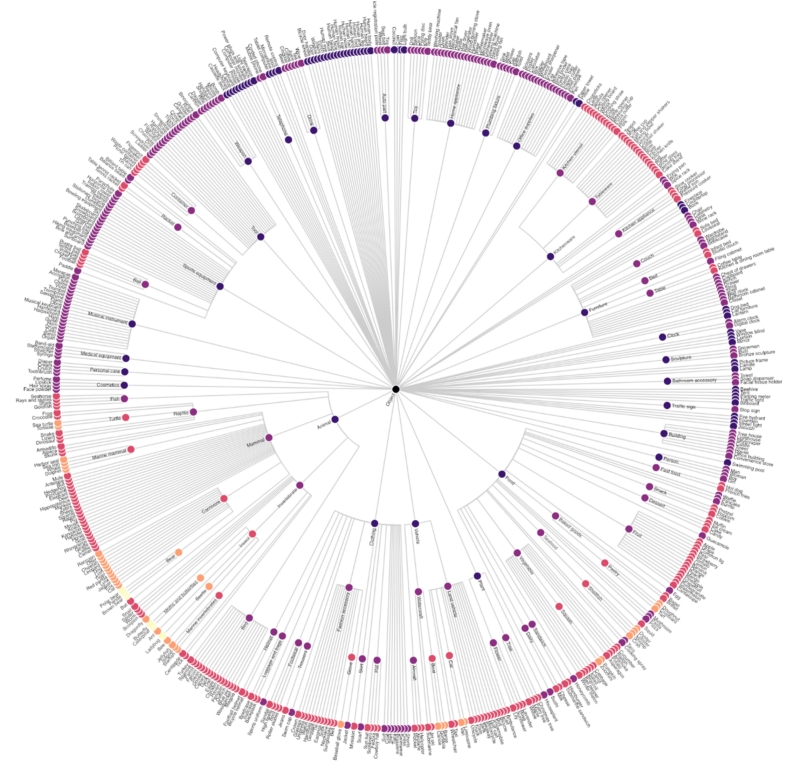
You can view an interactive annotated version of this chart (and download the code behind it) here.
Not all categories in Open Images have bounding box data associated with them.
But this script will allow you to download any subset of the 600 labels that do. Here’s a taste of what’s possible:
football, toy, bird, cat, vase, hair dryer, kangaroo, knife, briefcase, pencil case, tennis ball, nail, high heels, sushi, skyscraper, tree, truck, violin, wine, wheel, whale, pizza cutter, bread, helicopter, lemon, dog, elephant, shark, flower, furniture, airplane, spoon, bench, swan, peanut, camera, flute, helmet, pomegranate, crown…
For the purposes of this article, we’ll limit ourselves to just two: hamburger and sandwich.
Clean it, crop it
Once we’ve run the script and localized the images, we can inspect them with matplotlib to see what we’ve got:
import matplotlib.pyplot as pltfrom matplotlib.image import imread%matplotlib inlineimport os
fig, axarr = plt.subplots(1, 5, figsize=(24, 4))for i, img in enumerate(os.listdir('../data/images/')[:5]): axarr[i].imshow(imread('../data/images/' + img))
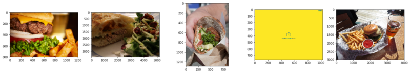 Five example {hamburger, sandwich} images from Google Open Images V4.
These images are not easy ones to train on. They have all of the issues associated with building a dataset using an external source from the public Internet.
Just this small sample here demonstrates the different sizes, orientations, and occlusions possible in our target classes.
In one case, we didn’t even succeed in downloading the actual image. Instead, we got a placeholder telling us that the image we wanted has since been deleted!
Downloading this data nets us a few thousand sample images like these. The next step is to take advantage of the bounding box information to clip our images down to just the sandwich-y, hamburger-y parts.
Here’s another image array, this time with bounding boxes included, to demonstrate what this entails:
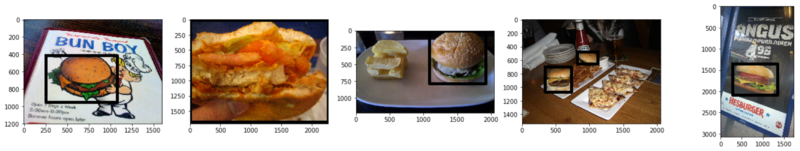 Bounding boxes. Notice (1) the dataset includes “depictions” and (2) raw images can contain many object instances.
This annotated Jupyter notebook in the demo GitHub repository does this work.
I will omit showing that code here because it is slightly complicated. This is especially since we also need to (1) refactor our image metadata to match the clipped image outputs and (2) extract the images that have since been deleted. Definitely check out the notebook if you wish to see the code.
After running the notebook code, we will have an images_cropped folder on disk containing all of the cropped images.
Building the model
Once we have downloaded the data, and cropped and cleaned it, we’re ready to train the model.
We will train a convolutional neural network (or ‘CNN’) on the data.
CNNs are a special type of neural network which build progressively higher level features out of groups of pixels commonly found in the images.
How an image scores on these various features is then weighted to generate a final classification result.
This architecture works extremely well because it takes advantage of locality. This is because any one pixel is likely to have far more in common with pixels nearby than those far away.
CNNs also have other attractive properties, like noise tolerance and scale invariance (to an extent). These further improve their classification properties.
If you’re unfamiliar with CNNs, I recommend skimming Brandon Rohrer’s excellent “How convolutional neural networks work” to learn more about them.
We will train a very simple convolutional neural network and see how even that gets decent results on our problem. I use Keras to define and train the model.
We start by laying out the images in a certain directory structure:
images_cropped/ sandwich/ some_image.jpg some_other_image.jpg ... hamburger/ yet_another_image.jpg ...
We then point Keras at this folder using the following code:
Keras will inspect the input folders, and determine there are two classes in our classification problem. It will assign class names based on the subfolder names, and create “image generators” that serve out of those folders.
But we don’t just return the images themselves. Instead, we return randomly subsampled, skewed, and zoomed selections from the images (via train_datagen.flow_from_directory).
This is an example of data augmentation in action.
Data augmentation is the practice of feeding an image classifier randomly cropped and distorted versions of an input dataset. This helps us overcome the small size of our dataset. We can train our model on a single image multiple times. Each time we use a slightly different segment of the image preprocessed in a slightly different way.
With our data input defined, the next step is defining the model itself:
This is a simple convolutional neural network model. It contains just three convolutional layers: a single densely connected post-processing layer just before the output layer, and strong regularization in the form of a dropout layer and relu activation.
These things all work together to make it more difficult for this model to overfit. This is important, given the small size of our input dataset.
Finally, the last step is actually fitting the model.
This code selects an epoch step size determined by our image sample size and chosen batch size (16). Then it trains on that data for 50 epochs.
Training is likely to be suspended early by the EarlyStopping callback. This returns the best performing model ahead of the 50 epoch limit if it does not see improvement in the validation score in the previous four epochs.
We selected such a large patience value because there is a significant amount of variability in model validation loss.
This simple training regimen results in a model with about 75% accuracy:
precision recall f1-score support 0 0.90 0.59 0.71 1399 1 0.64 0.92 0.75 1109 micro avg 0.73 0.73 0.73 2508 macro avg 0.77 0.75 0.73 2508weighted avg 0.78 0.73 0.73 2508
It’s interesting to note that our model is under-confident when classifying hamburgers (class 0), but over-confident when classifying hamburgers (class 1).
90% of images classified as hamburgers are actually hamburgers. But only 59% of all actual hamburgers are classified correctly.
On the other hand, just 64% of images classified as sandwiches are actually sandwiches. But 92% of sandwiches are classified correctly.
These results are in line with the 80% accuracy Francois Chollet got by applying a very similar model to a similarly-sized subset of the classic Cats versus Dogs dataset.
The difference is probably mainly due to increased level of occlusion and noise in the Google Open Images V4 dataset.
The dataset also includes illustrations as well as photographic images. These sometimes take large artistic liberties, making classification more difficult. You may choose to remove these when building a model yourself.
This performance can be further improved using transfer learning techniques. To learn more, check out Keras author Francois Chollet’s blog post “Building powerful image classification models using very little data”.
Distributing the model
Now that we’ve now built a custom dataset and trained a model, it’d be a shame if we didn’t share it.
Machine Learning projects should be reproducible. I outline the following strategy in a previous article, “Reproduce a machine learning model build in four lines of code”.
- Separate dependencies into data, code, and environment components.
- Data dependencies version control (1) the model definition and (2) the training data. Save these to versioned blob storage, e.g. Amazon S3 with Quilt T4.
- Code dependencies version controls the code used to train the model (use git).
- Environment dependencies version control the environment used to train the model. In a production environment this should probably be a Docker file, but you can use
piporcondalocally. - To provide someone with a retrainable copy of the model, give them the corresponding
{data, code, environment}tuple.
Following these principles makes getting everything you need to train your own copy of this model fit into a handful of lines of code:
git clone https://github.com/quiltdata/open-images.gitconda env create -f open-images/environment.ymlsource activate quilt-open-images-devpython -c "import t4; t4.Package.install('quilt/open_images', dest='open-images/', registry='s3://quilt-example')"
To learn more about {data, code, environment} see the GitHub repository and/or the corresponding article.
Conclusion
In this article we demonstrated an end-to-end image classification machine learning pipeline. We covered everything from downloading/transforming a dataset to training a model. We then distributed it in a way that lets anyone else rebuild it themselves later.
Because custom datasets are difficult to generate and distribute, over time there has emerged a cabal of example datasets which get used everywhere. This is not because they’re actually that good (they’re not). Instead, it’s because they’re easy.
For example, Google’s recently released Machine Learning Crash Course makes heavy use of the California Housing Dataset. That data is now almost two decades old!
Consider instead exploring new horizons. Using real images from the living Internet with interesting categorical breakdowns. It’s easier than you think!