

An Excel worksheet can be difficult to work with if it contains duplicates – especially if you’re not the author of the worksheet.
If you find them, you might want to highlight or remove such duplicates in the Excel sheet so you don’t run into errors.
In this article, I will show you 2 ways you can remove duplicates in your Excel worksheets.
How to Find and Remove Duplicates with Conditional Formatting
If you need to selectively remove some duplicates (but leave others), this is the method to use. Here's how it works:
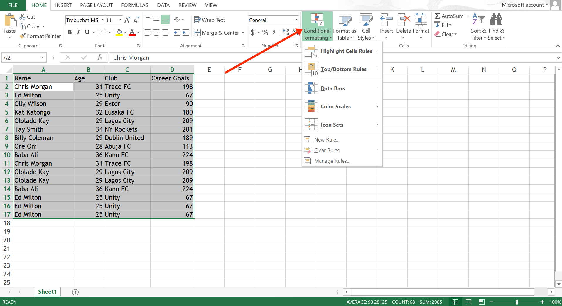
Step 1: Press CTRL + A to highlight the entire table, switch to the Home tab, then click on “Conditional Formatting”.
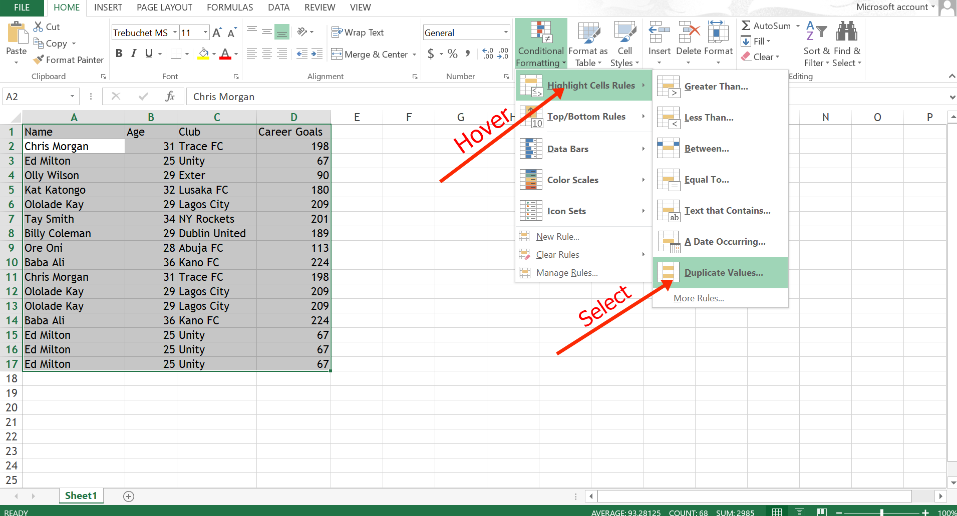
Step 2: Hover over “Highlight Cell Rules” and select “Duplicate Values”.
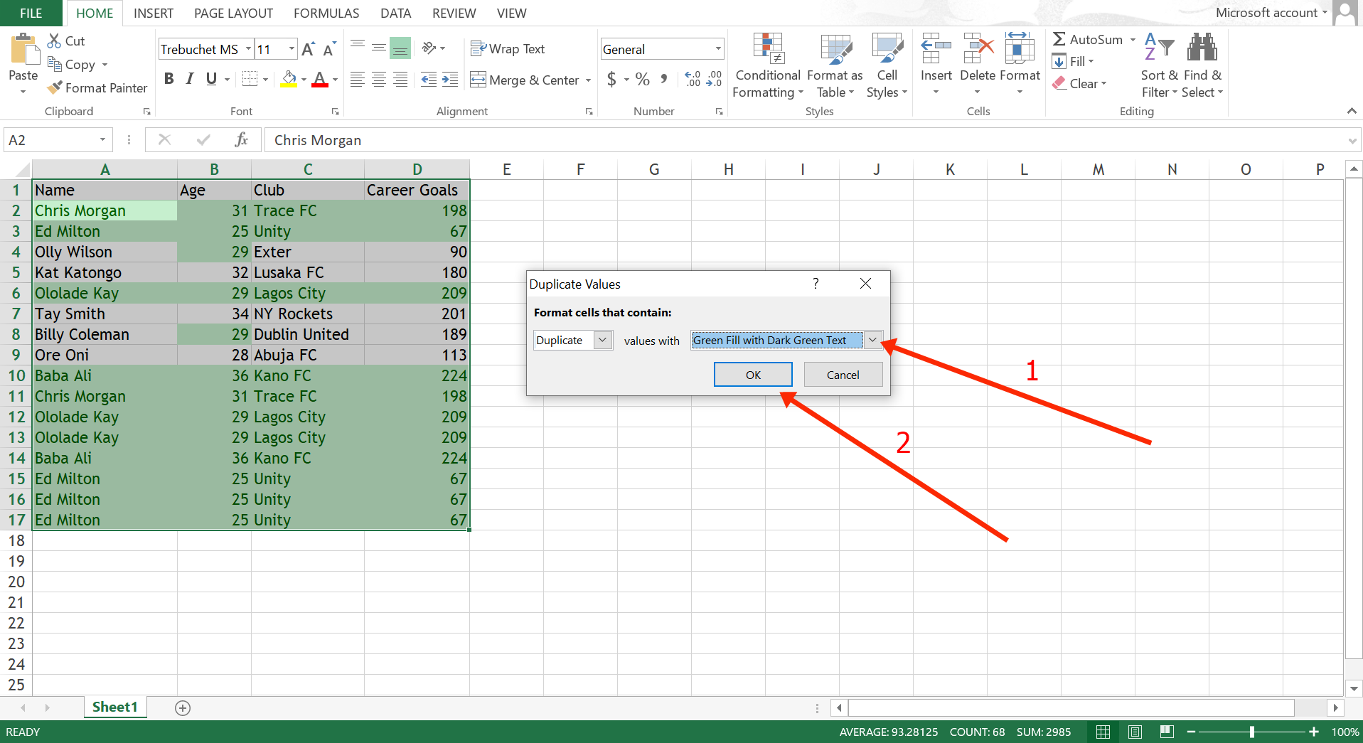
Step 3: Select how you want the duplicates to be highlighted, then click “Ok”.
Duplicate cells will now be highlighted for you so you can remove the ones you don’t need:
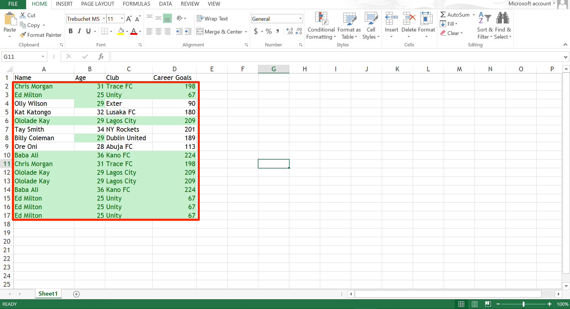
Again, on some occasions, you will need some duplicate entries. This method does not remove the duplicates automatically so you can do it yourself.
The next method removes duplicates automatically.
How to Remove Duplicates with the Remove Duplicate Command
This is one of the most reliable and straightforward ways to remove duplicates.
To use this method, follow the steps below:
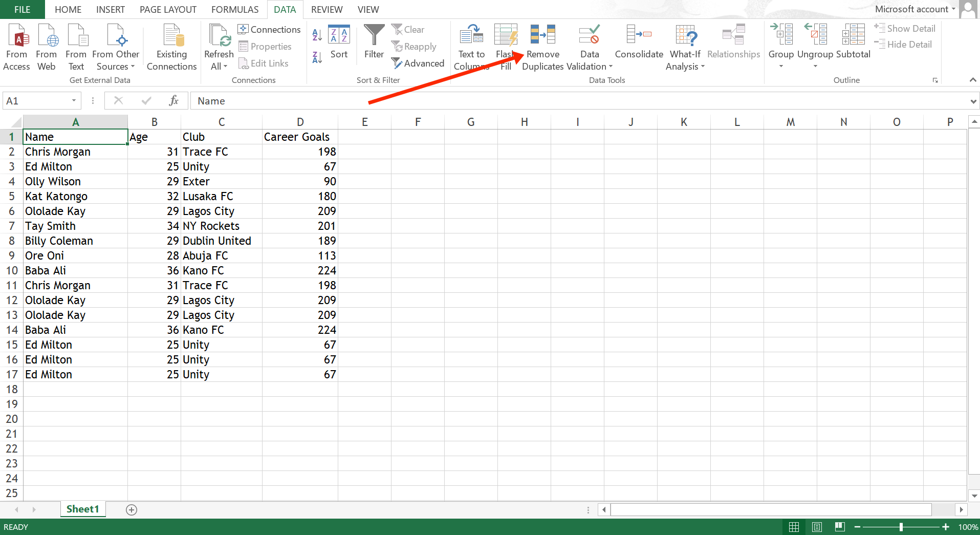
Step 1: Switch to the Data tab and click on “Remove Duplicates”.
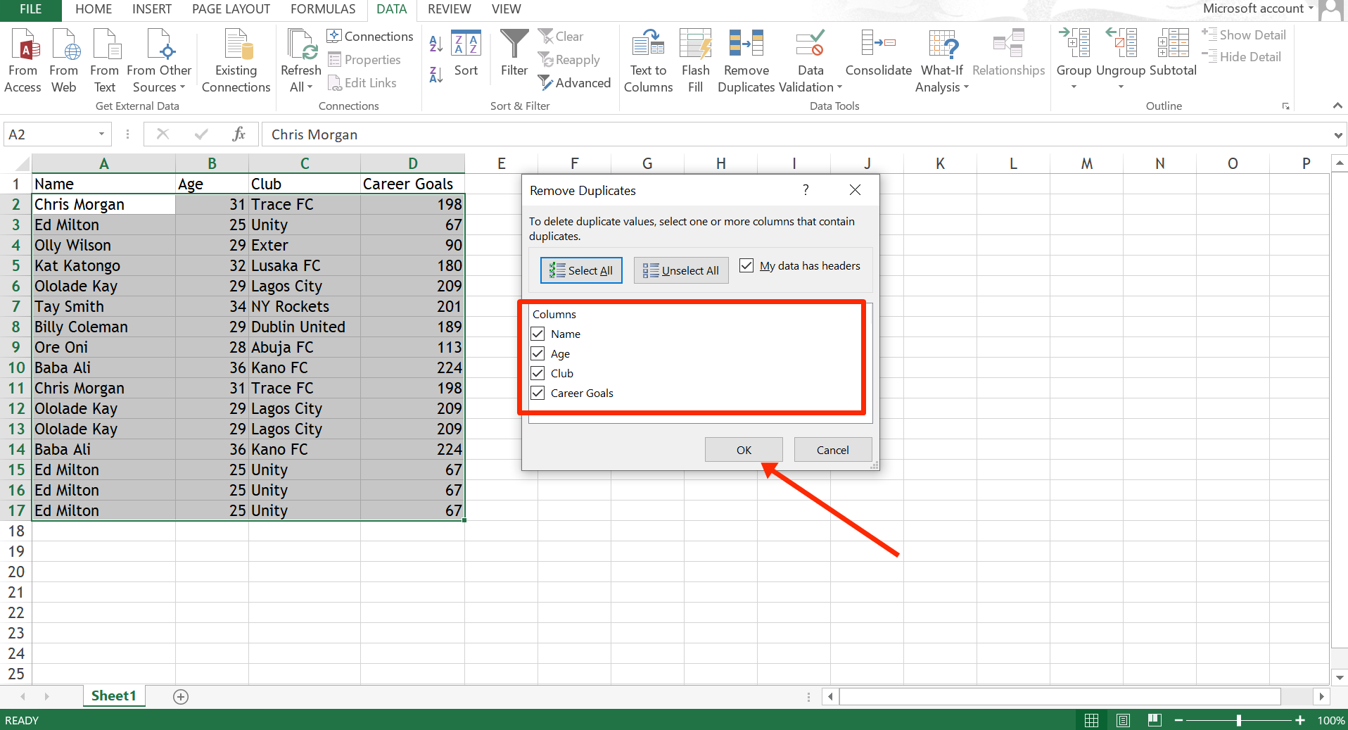
Step 2: Select all the columns in the table so Excel can look through and check for duplicates, then click “Ok”.
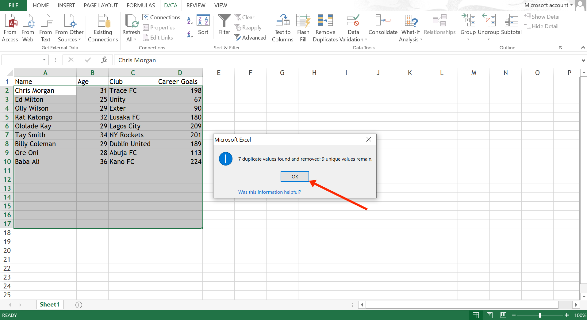
Step 3: You will get a message that duplicates have been removed. Click “Ok” to get rid of the message.
Conclusion
Duplicates can be a bottleneck for your productivity in Excel. Now that you know how to remove duplicates you can keep working effectively.
If this article helped you out, consider sharing it with your friends and family.
Thank you for reading.