by Hari Santanam

How to use Spark clusters for parallel processing Big Data

Use Apache Spark’s Resilient Distributed Dataset (RDD) with Databricks

Due to physical limitations, the individual computer processor has largely reached the upper ceiling for speed with current designs. So, hardware makers added more processors to the motherboard (parallel CPU cores, running at the same speed).

But… most software applications written over the last few decades were not written for parallel processing.

Additionally, data collection has gotten exponentially bigger, due to cheap devices that can collect specific data (such as temperature, sound, speed…).

To process this data in a more efficient way, newer programming methods were needed.

A cluster of computing processes is similar to a group of workers. A team can work better and more efficiently than a single worker. They pool resources. This means they share information, break down the tasks and collect updates and outputs to come up with a single set of results.

Just as farmers went from working on one field to working with combines and tractors to efficiently produce food from larger and more farms, and agricultural cooperatives made processing easier, the cluster works together to tackle larger and more complex data collection and processing.

Cluster computing and parallel processing were the answers, and today we have the Apache Spark framework. Databricks is a unified analytics platform used to launch Spark cluster computing in a simple and easy way.

What is Spark?

Apache Spark is a lightning-fast unified analytics engine for big data and machine learning. It was originally developed at UC Berkeley.

Spark is fast. It takes advantage of in-memory computing and other optimizations. It currently holds the record for large-scale on-disk sorting.

Spark uses Resilient Distributed Datasets (RDD) to perform parallel processing across a cluster or computer processors.

It has easy-to-use APIs for operating on large datasets, in various programming languages. It also has APIs for transforming data, and familiar data frame APIs for manipulating semi-structured data.

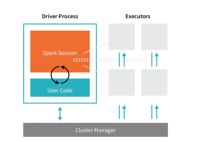
Basically, Spark uses a cluster manager to coordinate work across a cluster of computers. A cluster is a group of computers that are connected and coordinate with each other to process data and compute.

Spark applications consist of a driver process and executor processes.

Briefly put, the driver process runs the main function, and analyzes and distributes work across the executors. The executors actually do the tasks assigned — executing code and reporting to the driver node.

In real-world applications in business and emerging AI programming, parallel processing is becoming a necessity for efficiency, speed and complexity.

Great — so what is Databricks?

Databricks is a unified analytics platform, from the creators of Apache Spark. It makes it easy to launch cloud-optimized Spark clusters in minutes.

Think of it as an all-in-one package to write your code. You can use Spark (without worrying about the underlying details) and produce results.

It also includes Jupyter notebooks that can be shared, as well as providing GitHub integration, connections to many widely used tools and automation monitoring, scheduling and debugging. See here for more information.

You can sign up for free with the community edition. This will allow you to play around with Spark clusters. Other benefits, depending on plan, include:

• Get clusters up and running in seconds on both AWS and Azure CPU and GPU instances for maximum flexibility.
• Get started quickly with out-of-the-box integration of TensorFlow, Keras, and their dependencies on Databricks clusters.

Let’s get started. If you have already used Databricks before, skip down to the next part. Otherwise, you can sign up here and select ‘community edition’ to try it out for free.

Follow the directions there. They are clear, concise and easy:

• Create a cluster
• Attach a notebook to the cluster and run commands in the notebook on the cluster
• Manipulate the data and create a graph
• Operations on Python DataFrame API; create a DataFrame from a Databricks dataset
• Manipulate the data and display results

Now that you have created a data program on cluster, let’s move on to another dataset, with more operations so you can have more data.

The dataset is the 2017 World Happiness Report by country, based on different factors such as GDP, generosity, trust, family, and others. The fields and their descriptions are listed further down in the article.

I previously downloaded the dataset, then moved it into Databricks’ DBFS (DataBricks Files System) by simply dragging and dropping into the window in Databricks.

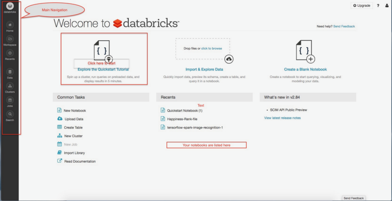
Or, you can click on Data from left Navigation pane, Click on Add Data, then either drag and drop or browse and add.

# File location and type#this file was dragged and dropped into Databricks from stored #location; https://www.kaggle.com/unsdsn/world-happiness#2017.csv 

file_location = "/FileStore/tables/2017.csv"file_type = "csv"

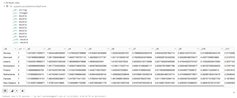
# CSV options# The applied options are for CSV files. For other file types, these # will be ignored: Schema is inferred; first row is header - I # deleted header row in editor and intentionally left it 'false' to #contrast with later rdd parsing, #delimiter # separated, #file_location; if you don't delete header row, instead of reading #C0, C1, it would read "country", "dystopia" etc.infer_schema = "true"first_row_is_header = "false"delimiter = ","df = spark.read.format(file_type) \  .option("inferSchema", infer_schema) \  .option("header", first_row_is_header) \  .option("sep", delimiter) \  .load(file_location)

display(df)

Now, let’s load the file into Spark’s Resilient Distributed Dataset(RDD) mentioned earlier. RDD performs parallel processing across a cluster or computer processors and makes data operations faster and more efficient.

#load the file into Spark's Resilient Distributed Dataset(RDD)data_file = "/FileStore/tables/2017.csv"raw_rdd = sc.textFile(data_file).cache()#show the top 5 lines of the fileraw_rdd.take(5)

Note the “Spark Jobs” below, just above the output. Click on View to see details, as shown in the inset window on the right.

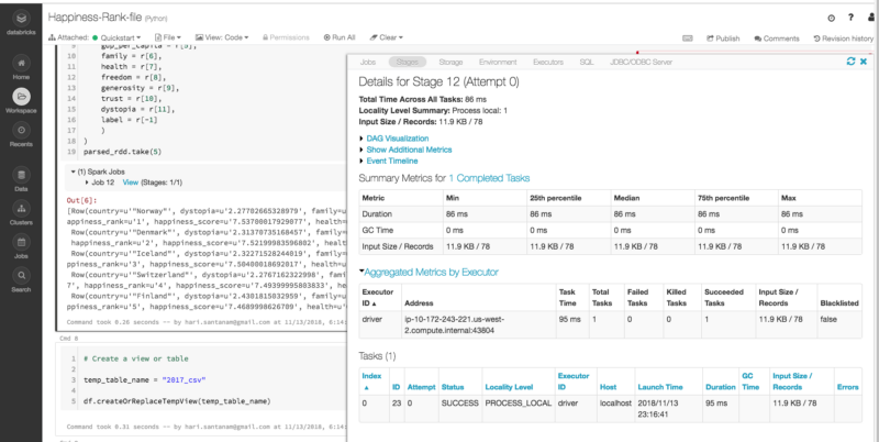
Databricks and Sparks have excellent visualizations of the processes.

In Spark, a job is associated with a chain of RDD dependencies organized in a direct acyclic graph (DAG). In a DAG, branches are directed from one node to another, with no loop backs. Tasks are submitted to the scheduler, which executes them using pipelining to optimize the work and transform into minimal stages.

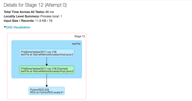
Don’t worry if the above items seem complicated. There are visual snapshots of processes occurring during the specific stage for which you pressed Spark Job view button. You may or may not need this information — it is there if you do.

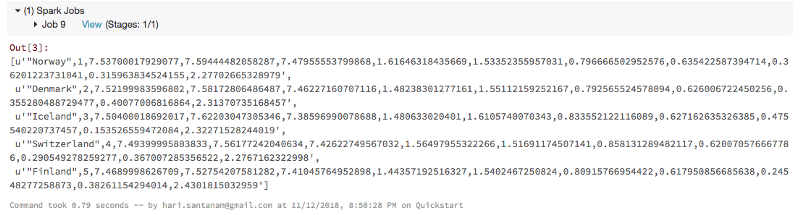
RDD entries are separated by commas, which we need to split before parsing and building a dataframe. We will then take specific columns from the dataset to use.

#split RDD before parsing and building dataframecsv_rdd = raw_rdd.map(lambda row: row.split(","))#print 2 rowsprint(csv_rdd.take(2))#print typesprint(type(csv_rdd))print('potential # of columns: ', len(csv_rdd.take(1)[0]))

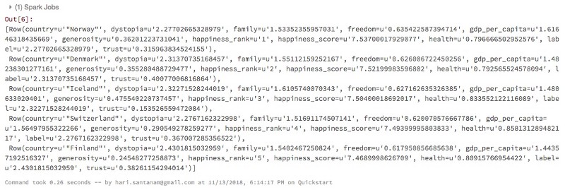
#use specific columns from dataset

from pyspark.sql import Row

parsed_rdd = csv_rdd.map(lambda r: Row(    country = r[0],   #country, position 1, type=string    happiness_rank = r[1],    happiness_score = r[2],    gdp_per_capita = r[5],    family = r[6],    health = r[7],    freedom = r[8],    generosity = r[9],    trust = r[10],    dystopia = r[11],    label = r[-1]    ))parsed_rdd.take(5)

Here are the columns and definitions for the Happiness dataset:

Happiness dataset columns and definitions

Country — Name of the country.

Region — Region the country belongs to.

Happiness Rank — Rank of the country based on the Happiness Score.

Happiness Score — A metric measured in 2015 by asking the sampled people the question: “How would you rate your happiness on a scale of 0 to 10 where 10 is the happiest.”

Economy (GDP per Capita) — The extent to which GDP (Gross Domestic Product) contributes to the calculation of the Happiness Score

Family — The extent to which Family contributes to the calculation of the Happiness Score

Health — (Life Expectancy)The extent to which Life expectancy contributed to the calculation of the Happiness Score

Freedom — The extent to which Freedom contributed to the calculation of the Happiness Score.

Trust — (Government Corruption)The extent to which Perception of Corruption contributes to Happiness Score.

Generosity — The extent to which Generosity contributed to the calculation of the Happiness Score.

Dystopia Residual — The extent to which Dystopia Residual contributed to the calculation of the Happiness Score (Dystopia=imagined place or state in which everything is unpleasant or bad, typically a totalitarian or environmentally degraded one. Residual — what’s left or remaining after everything is else is accounted for or taken away).

# Create a view or table

temp_table_name = "2017_csv"

df.createOrReplaceTempView(temp_table_name)

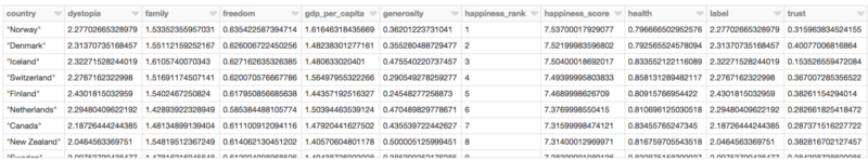
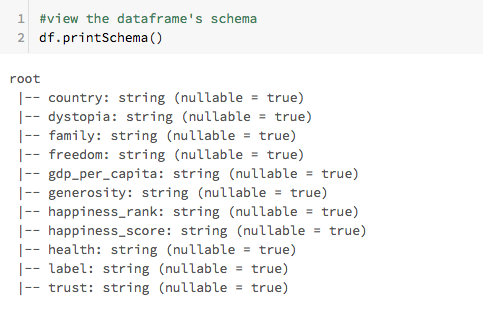
#build dataframe from RDD created earlierdf = sqlContext.createDataFrame(parsed_rdd)display(df.head(10)#view the dataframe's schemadf.printSchema()

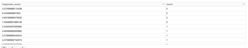
#build temporary table to run SQL commands#table only alive for the session#table scoped to the cluster; highly optimizeddf.registerTempTable("happiness")#display happiness_score counts using dataframe syntaxdisplay(df.groupBy('happiness_score')          .count()          .orderBy('count', ascending=False)       )

df.registerTempTable("happiness")

#display happiness_score counts using dataframe syntaxdisplay(df.groupBy('happiness_score')          .count()          .orderBy('count', ascending=False)       )

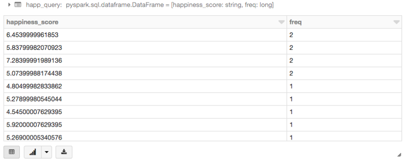
Now, let’s use SQL to run a query to do same thing. The purpose is to show you different ways to process data and to compare the methods.

#use SQL to run query to do same thing as previously done with dataframe (count by happiness_score)happ_query = sqlContext.sql("""                        SELECT happiness_score, count(*) as freq                        FROM happiness                        GROUP BY happiness_score                        ORDER BY 2 DESC                        """)display(happ_query)

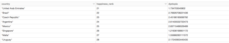
Another SQL query to practice our data processing:

#another sql queryhapp_stats = sqlContext.sql("""                            SELECT                              country,                              happiness_rank,                              dystopia                            FROM happiness                            WHERE happiness_rank > 20                            """)display(happ_stats)

There! You have done it — created a Spark-powered cluster and completed a dataset query process using that cluster. You can use this with your own datasets to process and output your Big Data projects.

You can also play around with the charts-click on the chart /graph icon at the bottom of any output, specify the values and type of graph and see what happens. It is fun.

The code is posted in a notebook here at Databricks public forum and will be available for about 6 months as per Databricks.

• For more information on using Sparks with Deep Learning, read this excellent article by Favio Vázquez

Thanks for reading! I hope you have interesting programs with Databricks and enjoy it as much as I have. Please clap if you found it interesting or useful.

For a complete list of my articles, see here.