
Welcome! If you want to start diving into data science and statistics, then data frames, CSV files, and R will be essential tools for you. Let's see how you can use their amazing capabilities.
In this article, you will learn:
- What CSV files are and what they are used for.
- How to create CSV files using Google Sheets.
- How to read CSV files in R.
- What Data Frames are and what they are used for.
- How to access the elements of a data frame.
- How to modify a data frame.
- How to add and delete rows and columns.
We will use RStudio, an open-source IDE (Integrated Development Environment) to run the examples.
Let's begin! ✨
🔹 Introduction to CSV Files
CSV (Comma-separated Values) files can be considered one of the building blocks of data analysis because they are used to store data represented in the form of a table.
In this file, values are separated by commas to represent the different columns of the table, like in this example:
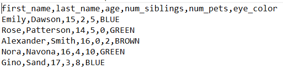 CSV File
We will generate this file using Google Sheets.
🔸 How to Create a CSV File Using Google Sheets
Let's create your first CSV file using Google Sheets.
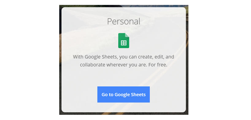
Step 1: Go to the Google Sheets Website and click on "Go to Google Sheets":
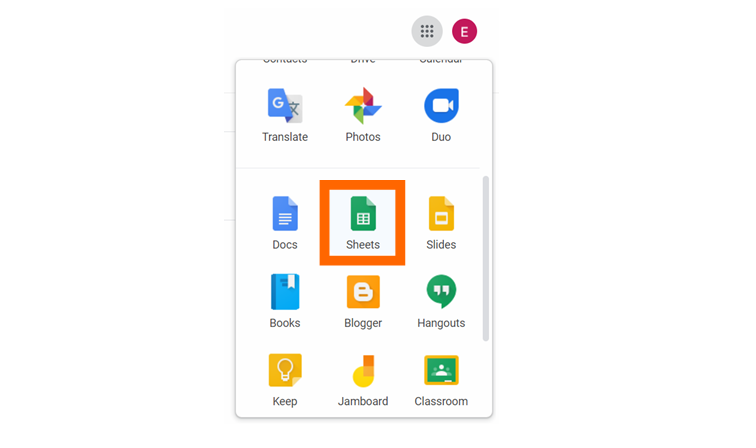
💡 Tip: You can access Google Sheets by clicking on the button located at the top-right edge of Google's Home Page:

If we zoom in, we see the "Sheets" button:
💡 Tip: To use Google Sheets, you need to have a Gmail account. Alternatively, you can create a CSV file using MS Excel or another spreadsheet editor.
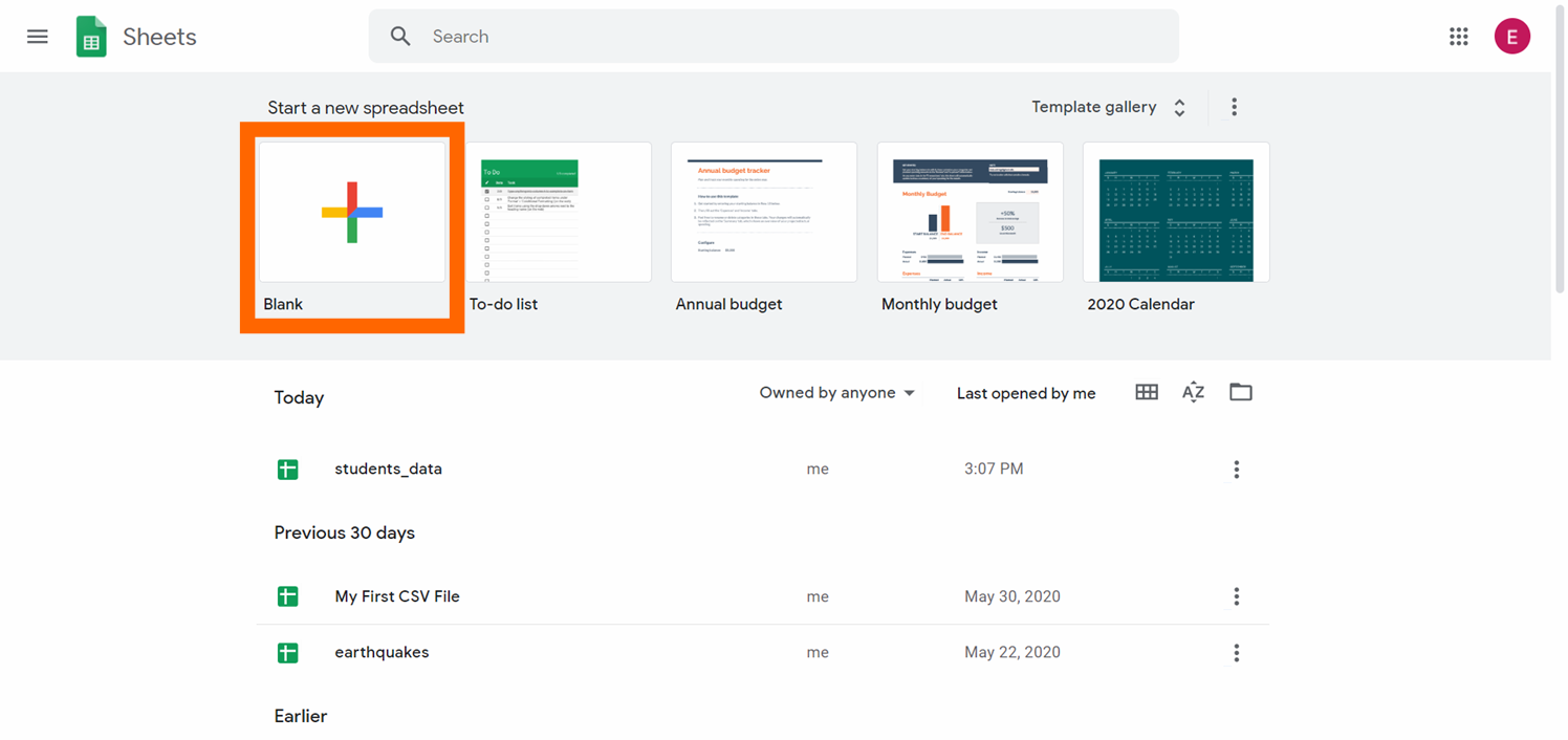
You will see this panel:
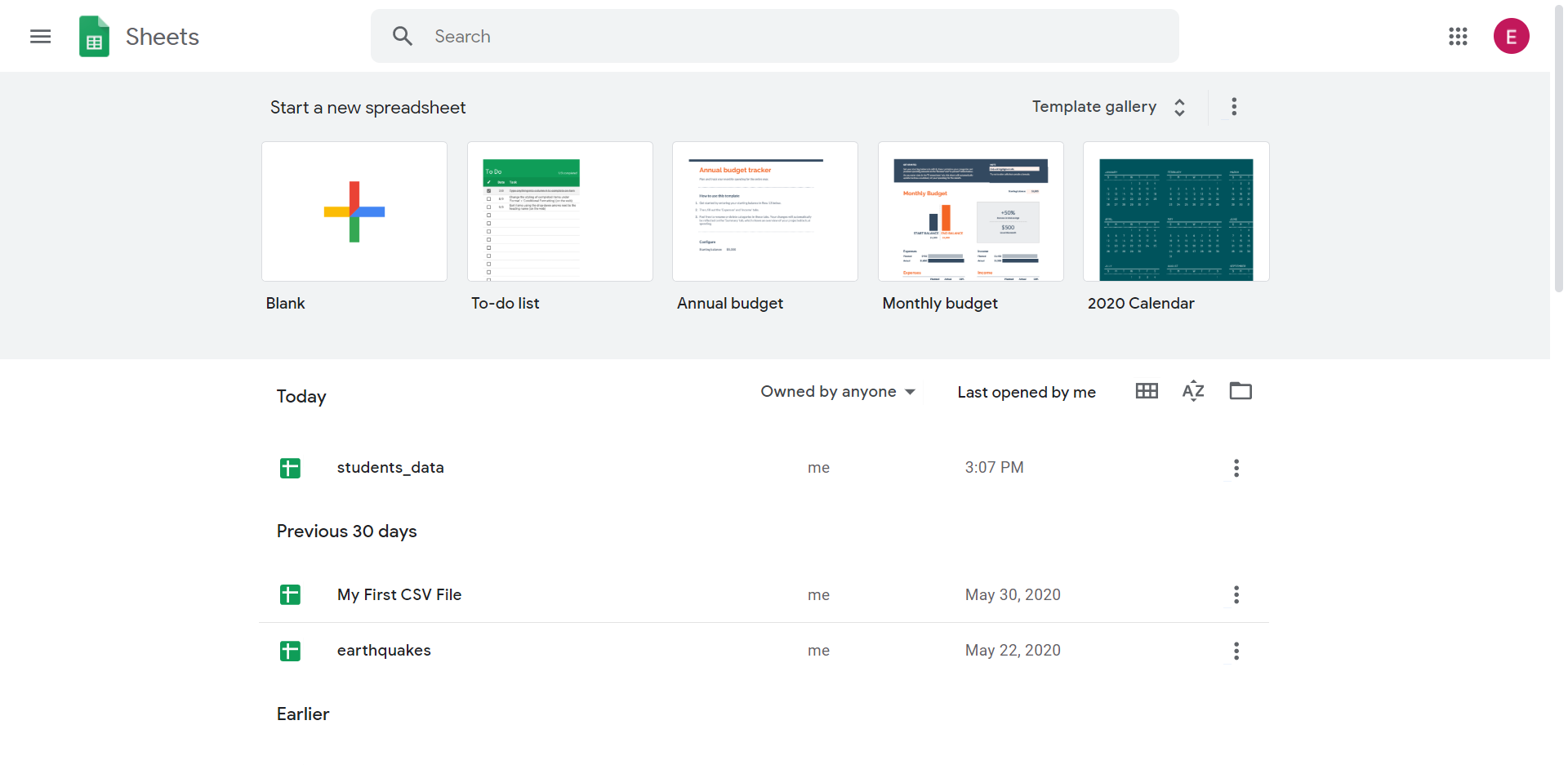
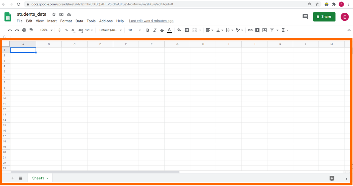
Step 2: Create a blank spreadsheet by clicking on the "+" button.
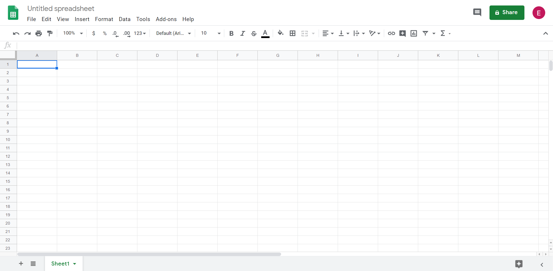
Now you have a new empty spreadsheet:
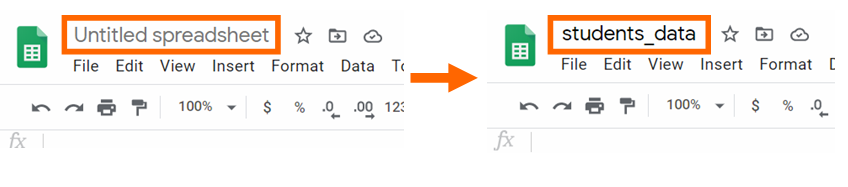
Step 3: Change the name of the spreadsheet to students_data. We will need to use the name of the file to work with data frames. Write the new name and click enter to confirm the change.
Step 4: In the first row of the spreadsheet, write the titles of the columns.
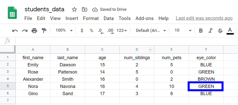
When you import a CSV file in R, the titles of the columns are called variables. We will define six variables: first_name, last_name, age, num_siblings, num_pets, and eye_color, as you can see right here below:
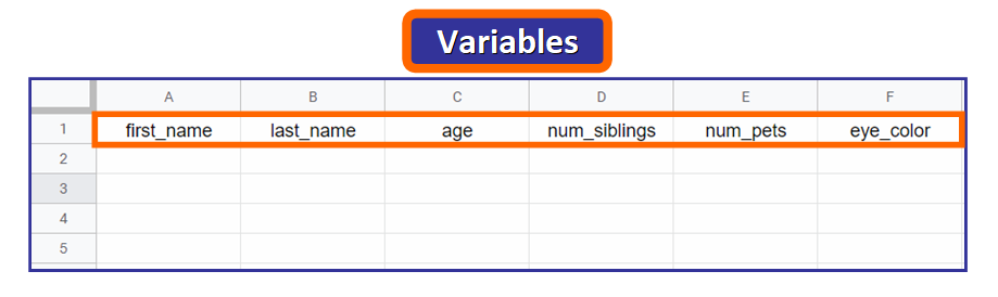
💡 Tip: Notice that the names are written in lowercase and words are separated with an underscore. This is not mandatory, but since you will need to access these names in R, it's very common to use this format.
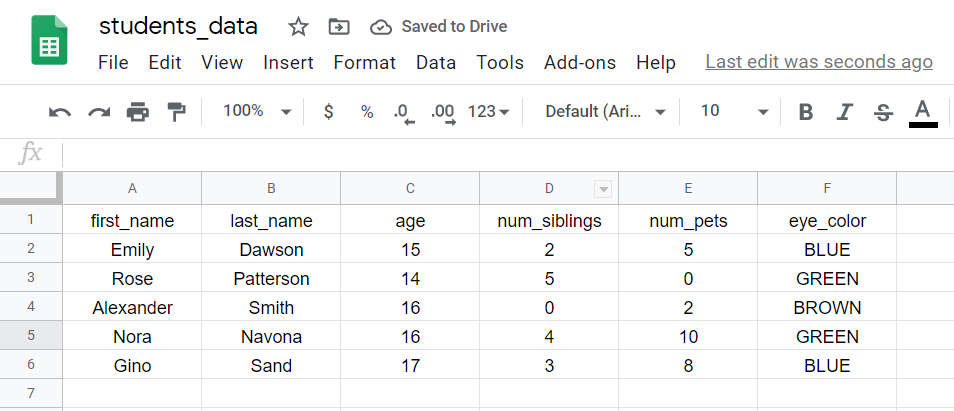
Step 5: Enter the data for each one of the columns.
When you read the file in R, each row is called an observation, and it corresponds to data taken from an individual, animal, object, or entity that we collected data from.
In this case, each row corresponds to the data of a student:
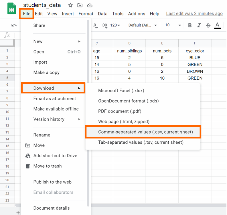
Step 6: Download the CSV file by clicking on File -> Download -> Comma-separated values, as you can see below:
Step 7: Rename the file CSV file. You will need to remove "Sheet1" from the default name because Google Sheet will automatically add this to the name of the file.

Great work! Now you have your CSV file and it's time to start working with it in R.
🔹 How to Read a CSV file in R
In RStudio, the first step before reading a CSV file is making sure that your current working directory is the directory where the CSV file is located.
💡 Tip: If this is not the case, you will need to use the full path to the file.
Change Current Working Directory
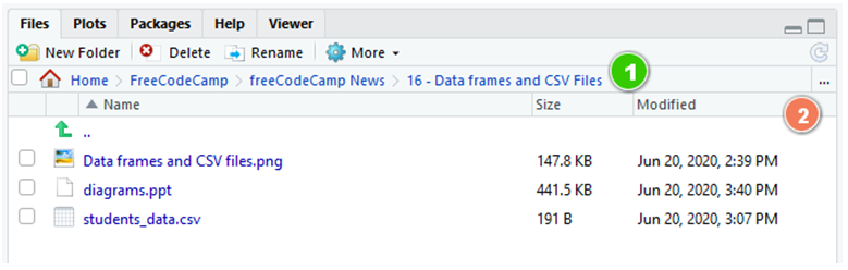
You can change your current working directory in this panel:
If we zoom in, you can see the current path (1) and select the new one by clicking on the ellipsis (...) button to the right (2):
💡 Tip: You can also check your current working directory with getwd() in the interactive console.
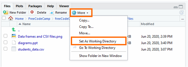
Then, click "More" and "Set As Working Directory".
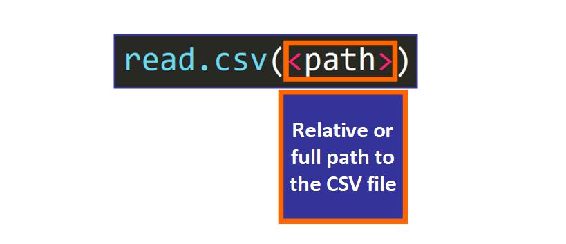
Read the CSV File
Once you have your current working directory set up, you can read the CSV file with this command:
In R code, we have this:
> students_data <- read.csv("students_data.csv")
💡 Tip: We assign it to the variable students_data to access the data of the CSV file with this variable. In R, we can separate words using dots ., underscores _, UpperCamelCase, or lowerCamelCase.
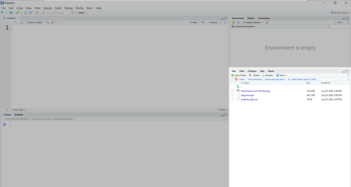
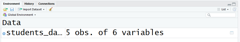
After running this command, you will see this in the top right panel:
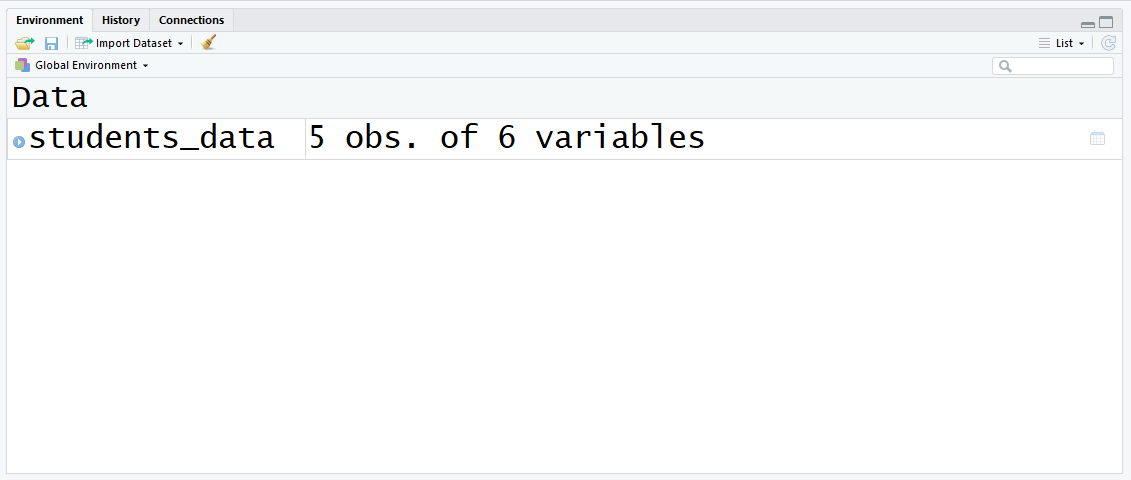
Now you have a variable defined in the environment! Let's see what data frames are and how they are closely related to CSV files.
🔸 Introduction to Data Frames
Data frames are the standard digital format used to store statistical data in the form of a table. When you read a CSV file in R, a data frame is generated.
We can confirm this by checking the type of the variable with the class function:
> class(students_data)
[1] "data.frame"
It makes sense, right? CSV files contain data represented in the form of a table and data frames represent that tabular data in your code, so they are deeply connected.
If you enter this variable in the interactive console, you will see the content of the CSV file:
> students_data
  first_name last_name age num_siblings num_pets eye_color
1      Emily    Dawson  15            2        5      BLUE
2       Rose Patterson  14            5        0     GREEN
3  Alexander     Smith  16            0        2     BROWN
4       Nora    Navona  16            4       10     GREEN
5       Gino      Sand  17            3        8      BLUE
More Information About the Data Frame
You have several different alternatives to see the number of variables and observations of the data frame:
- Your first option is to look at the top right panel that shows the variables that are currently defined in the environment. This data frame has 5 observations (rows) and 6 variables (columns):
- Another alternative is to use the functions
nrowandncolin the interactive console or in your program, passing the data frame as argument. We get the same results: 5 rows and 6 columns.
> nrow(students_data)
[1] 5
> ncol(students_data)
[1] 6
- You can also see more information about the data frame using the
strfunction:
> str(students_data)
'data.frame':    5 obs. of  6 variables:
 $ first_name  : Factor w/ 5 levels "Alexander","Emily",..: 2 5 1 4 3
 $ last_name   : Factor w/ 5 levels "Dawson","Navona",..: 1 3 5 2 4
 $ age         : int  15 14 16 16 17
 $ num_siblings: int  2 5 0 4 3
 $ num_pets    : int  5 0 2 10 8
 $ eye_color   : Factor w/ 3 levels "BLUE","BROWN",..: 1 3 2 3 1
This function (applied to a data frame) tells you:
- The number of observations (rows).
- The number of variables (columns).
- The names of the variables.
- The data types of the variables.
- More information about the variables.
You can see that this function is really great when you want to know more about the data that you are working with.
💡 Tip: In R, a "Factor" is a qualitative variable, which is a variable whose values represent categories. For example, eye_color has the values "BLUE", "BROWN", "GREEN" which are categories, so as you can see in the output of str above, this variable is automatically defined as a "factor" when the CSV file is read in R.
🔹 Data Frames: Key Operations and Functions
Now you know how to see more information about the data frame. But the magic of data frames lies in the amazing capabilities and functionality that they offer, so let's see this in more detail.
How to Access A Value of a Data Frame
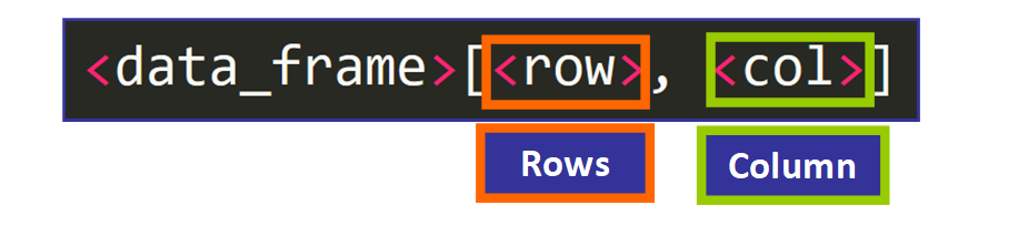
Data frames are like matrices, so you can access individual values using two indices surrounded by square brackets and separated by a comma to indicate which rows and which columns you would like to include in the result, like this:
For example, if we want to access the value of eye_color (column 6) of the fourth student in the data (row 4):
We need to use this command:
> students_data[4, 6]
💡 Tip: In R, indices start at 1 and the first row with the names of the variables is not counted.
This is the output:
[1] GREEN
Levels: BLUE BROWN GREEN
You can see that the value is "GREEN". Variables of type "factor" have "levels" that represent the different categories or values that they can take. This output tells us the levels of the variable eye_color.
How to Access Rows and Columns of a Data Frame
We can also use this syntax to access a range of rows and columns to get a portion of the original matrix, like this:
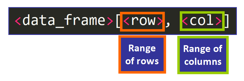
For example, if we want to get the age and number of siblings of the third, fourth, and fifth student in the list, we would use:
> students_data[3:5, 3:4]

  age num_siblings
3  16            0
4  16            4
5  17            3
💡 Tip: The basic syntax to define an interval in R is <start>:<end>. Note that these indices are inclusive, so the third and fifth elements are included in the example above when we write 3:5.
If we want to get all the rows or columns, we simply omit the interval and include the comma, like this:
> students_data[3:5,]

  first_name last_name age num_siblings num_pets eye_color
3  Alexander     Smith  16            0        2     BROWN
4       Nora    Navona  16            4       10     GREEN
5       Gino      Sand  17            3        8      BLUE
We did not include an interval for the columns after the comma in students_data[3:5,], so we get all the columns of the data frame for the three rows that we specified.
Similarly, we can get all the rows for a specific range of columns if we omit the rows:
> students_data[, 1:3]

  first_name last_name age
1      Emily    Dawson  15
2       Rose Patterson  14
3  Alexander     Smith  16
4       Nora    Navona  16
5       Gino      Sand  17
💡 Tip: Notice that you still need to include the comma in both cases.
How to Access a Column
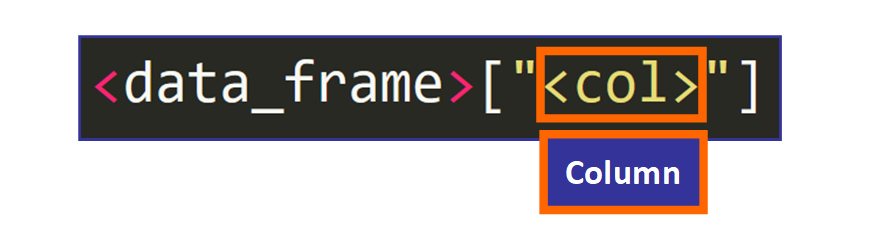
There are three ways to access an entire column:
- Option #1: to access a column and return it as a data frame, you can use this syntax:
For example:
> students_data["first_name"]

  first_name
1      Emily
2       Rose
3  Alexander
4       Nora
5       Gino
- Option #2: to get a column as a vector (sequence), you can use this syntax:
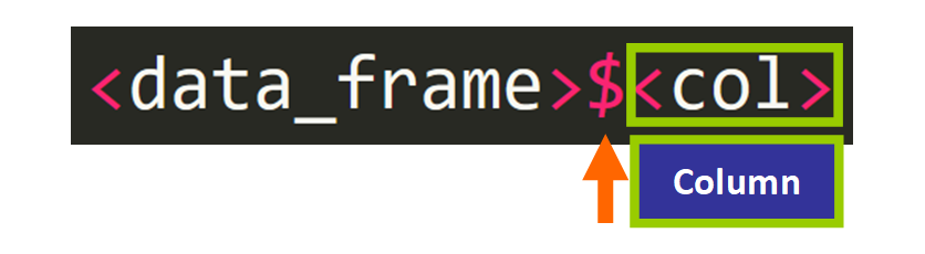
💡 Tip: Notice the use of the $ symbol.
For example:
> students_data$first_name

[1] Emily     Rose      Alexander Nora      Gino
Levels: Alexander Emily Gino Nora Rose
- Option #3: You can also use this syntax to get the column as a vector (see below). This is equivalent to the previous syntax:
> students_data[["first_name"]]

[1] Emily     Rose      Alexander Nora      Gino
Levels: Alexander Emily Gino Nora Rose
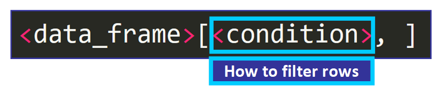
How to Filter Rows of a Data Frame
You can filter the rows of a data frame to get a portion of the matrix that meets certain conditions.
For this, we use this syntax, passing the condition as the first element within square brackets, then a comma, and finally leaving the second element empty.
For example, to get all rows for which students_data$age > 16, we would use:
> students_data[students_data$age > 16,]

  first_name last_name age num_siblings num_pets eye_color
5       Gino      Sand  17            3        8      BLUE
We get a data frame with the rows that meet this condition.
Filter Rows and Choose Columns
You can combine this condition with a range of columns:
> students_data[students_data$age > 16, 3:6]

  age num_siblings num_pets eye_color
5  17            3        8      BLUE
We get the rows that meet the condition and the columns in the range 3:6.
🔸 How to Modify Data Frames
You can modify individual values of a data frame, add columns, add rows, and remove them. Let's see how you can do this!
How to Change A Value
To change an individual value of the data frame, you need to use this syntax:
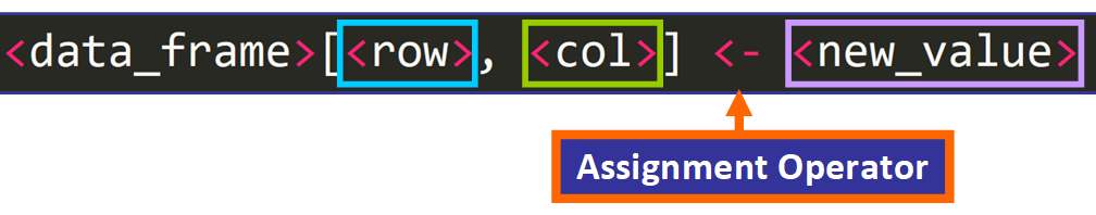
For example, if we want to change the value that is currently at row 4 and column 6, denoted in blue right here:
We need to use this line of code:
students_data[4, 6] <- "BROWN"
💡 Tip: You can also use = as the assignment operator.
This is the output. The value was changed successfully.
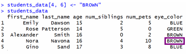
💡 Tip: Remember that the first row of the CSV file is not counted as the first row because it has the names of the variables.
How to Add Rows to a Data Frame
To add a row to a data frame, you need to use the rbind function:
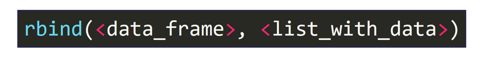
This function takes two arguments:
- The data frame that you want to modify.
- A list with the data of the new row. To create the list, you can use the
list()function with each value separated by a comma.
This is an example:
> rbind(students_data, list("William", "Smith", 14, 7, 3, "BROWN"))
The output is:
  first_name last_name age num_siblings num_pets eye_color
1      Emily    Dawson  15            2        5      BLUE
2       Rose Patterson  14            5        0     GREEN
3  Alexander     Smith  16            0        2     BROWN
4       Nora    Navona  16            4       10     BROWN
5       Gino      Sand  17            3        8      BLUE
6       <NA>     Smith  14            7        3     BROWN
But wait! A warning message was displayed:
Warning message:
In `[<-.factor`(`*tmp*`, ri, value = "William") :
  invalid factor level, NA generated
And notice the first value of the sixth row, it is <NA>:
6 <NA> Smith 14 7 3 BROWN
This occurred because the variable first_name was defined automatically as a factor when we read the CSV file and factors have fixed "categories" (levels).
You cannot add a new level (value - "William") to this variable unless you read the CSV file with the value FALSE for the parameter stringsAsFactors, as shown below:
> students_data <- read.csv("students_data.csv", stringsAsFactors = FALSE)

Now, if we try to add this row, the data frame is modified successfully.
> students_data <- rbind(students_data, list("William", "Smith", 14, 7, 3, "BROWN"))
> students_data

  first_name last_name age num_siblings num_pets eye_color
1      Emily    Dawson  15            2        5      BLUE
2       Rose Patterson  14            5        0     GREEN
3  Alexander     Smith  16            0        2     BROWN
4       Nora    Navona  16            4       10     GREEN
5       Gino      Sand  17            3        8      BLUE
6    William     Smith  14            7        3     BROWN
💡 Tip: Note that if you read the CSV file again and assign it to the same variable, all the changes made previously will be removed and you will see the original data frame. You need to add this argument to the first line of code that reads the CSV file and then make changes to it.
How to Add Columns to a Data Frame
Adding columns to a data frame is much simpler. You need to use this syntax:

For example:
> students_data$GPA <- c(4.0, 3.5, 3.2, 3.15, 2.9, 3.0)
💡 Tip: The number of elements has to be equal to the number of rows of the data frame.
The output shows the data frame with the new GPA column:
> students_data

  first_name last_name age num_siblings num_pets eye_color  GPA
1      Emily    Dawson  15            2        5      BLUE 4.00
2       Rose Patterson  14            5        0     GREEN 3.50
3  Alexander     Smith  16            0        2     BROWN 3.20
4       Nora    Navona  16            4       10     GREEN 3.15
5       Gino      Sand  17            3        8      BLUE 2.90
6    William     Smith  14            7        3     BROWN 3.00
How to Remove Columns
To remove columns from a data frame, you need to use this syntax:
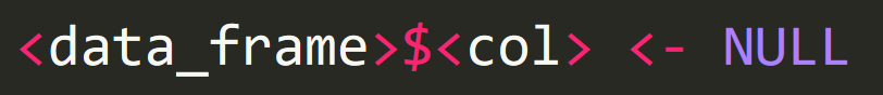
When you assign the value Null to a column, that column is removed from the data frame automatically.
For example, to remove the age column, we use:
> students_data$age <- NULL
The output is:
> students_data

  first_name last_name num_siblings num_pets eye_color  GPA
1      Emily    Dawson            2        5      BLUE 4.00
2       Rose Patterson            5        0     GREEN 3.50
3  Alexander     Smith            0        2     BROWN 3.20
4       Nora    Navona            4       10     GREEN 3.15
5       Gino      Sand            3        8      BLUE 2.90
6    William     Smith            7        3     BROWN 3.00
How to Remove Rows
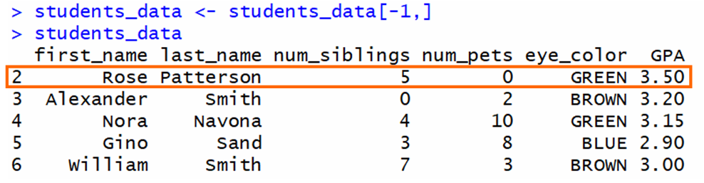
To remove rows from a data frame, you can use indices and ranges. For example, to remove the first row of a data frame:

The [-1,] takes a portion of the data frame that doesn't include the first row. Then, this portion is assigned to the same variable.
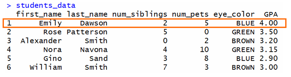
If we have this data frame and we want to delete the first row:
The output is a data frame that doesn't include the first row:
In general, to remove a specific row, you need to use this syntax where <row_num> is the row that you want to remove:

💡 Tip: Notice the - sign before the row number.
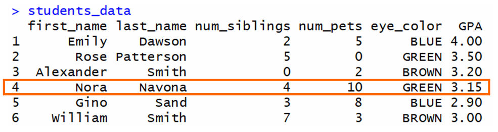
For example, if we want to remove row 4 from this data frame:
The output is:
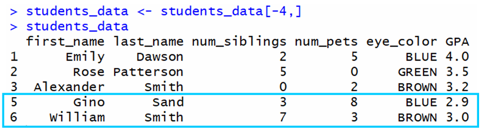
As you can see, row 4 was successfully removed.
🔹 In Summary
- CSV files are Comma-Separated Values Files used to represent data in the form of a table. These files can be read using R and RStudio.
- Data frames are used in R to represent tabular data. When you read a CSV file, a data frame is created to store the data.
- You can access and modify the values, rows, and columns of a data frame.
I really hope that you liked my article and found it helpful. Now you can work with data frames and CSV files in R.
If you liked this article, consider enrolling in my new online course "Introduction to Statistics in R - A Practical Approach"