By Thomas Simonini
This article is part of Deep Reinforcement Learning Course with Tensorflow ?️. Check the syllabus here.
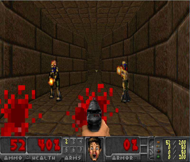
In our last article about Deep Q Learning with Tensorflow, we implemented an agent that learns to play a simple version of Doom. In the video version, we trained a DQN agent that plays Space invaders.
However, during the training, we saw that there was a lot of variability.
Deep Q-Learning was introduced in 2014. Since then, a lot of improvements have been made. So, today we’ll see four strategies that improve — dramatically — the training and the results of our DQN agents:
- fixed Q-targets
- double DQNs
- dueling DQN (aka DDQN)
- Prioritized Experience Replay (aka PER)
We’ll implement an agent that learns to play Doom Deadly corridor. Our AI must navigate towards the fundamental goal (the vest), and make sure they survive at the same time by killing enemies.
Fixed Q-targets
Theory
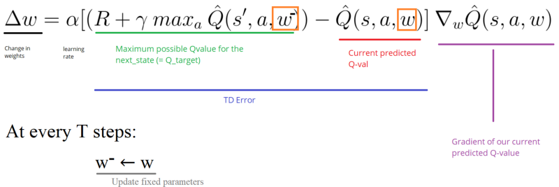
We saw in the Deep Q Learning article that, when we want to calculate the TD error (aka the loss), we calculate the difference between the TD target (Q_target) and the current Q value (estimation of Q).
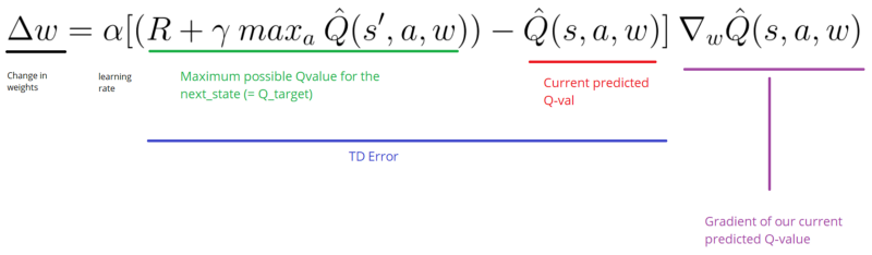
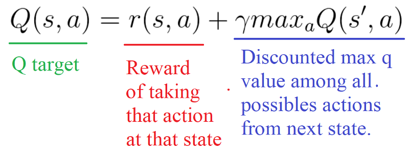
But we don’t have any idea of the real TD target. We need to estimate it. Using the Bellman equation, we saw that the TD target is just the reward of taking that action at that state plus the discounted highest Q value for the next state.
However, the problem is that we using the same parameters (weights) for estimating the target and the Q value. As a consequence, there is a big correlation between the TD target and the parameters (w) we are changing.
Therefore, it means that at every step of training, our Q values shift but also the target value shifts. So, we’re getting closer to our target but the target is also moving. It’s like chasing a moving target! This lead to a big oscillation in training.
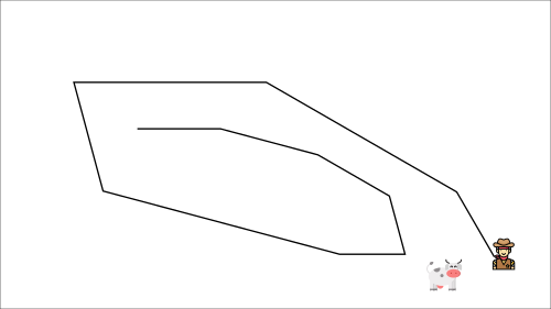
It’s like if you were a cowboy (the Q estimation) and you want to catch the cow (the Q-target) you must get closer (reduce the error).
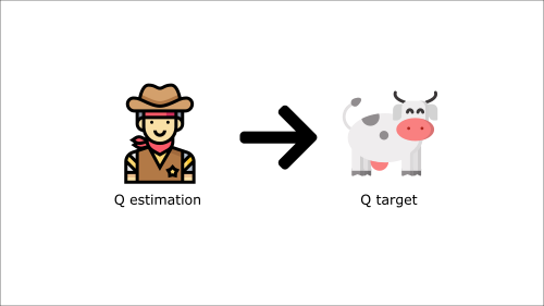
At each time step, you’re trying to approach the cow, which also moves at each time step (because you use the same parameters).

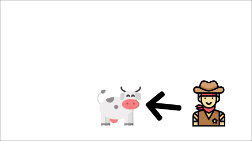
This leads to a very strange path of chasing (a big oscillation in training).
Instead, we can use the idea of fixed Q-targets introduced by DeepMind:
- Using a separate network with a fixed parameter (let’s call it w-) for estimating the TD target.
- At every Tau step, we copy the parameters from our DQN network to update the target network.
Thanks to this procedure, we’ll have more stable learning because the target function stays fixed for a while.
Implementation
Implementing fixed q-targets is pretty straightforward:
First, we create two networks (
DQNetwork,TargetNetwork)Then, we create a function that will take our
DQNetworkparameters and copy them to ourTargetNetworkFinally, during the training, we calculate the TD target using our target network. We update the target network with the
DQNetworkeverytaustep (tauis an hyper-parameter that we define).
Double DQNs
Theory
Double DQNs, or double Learning, was introduced by Hado van Hasselt. This method handles the problem of the overestimation of Q-values.
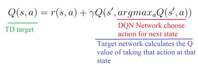
To understand this problem, remember how we calculate the TD Target:
By calculating the TD target, we face a simple problem: how are we sure that the best action for the next state is the action with the highest Q-value?
We know that the accuracy of q values depends on what action we tried and what neighboring states we explored.
As a consequence, at the beginning of the training we don’t have enough information about the best action to take. Therefore, taking the maximum q value (which is noisy) as the best action to take can lead to false positives. If non-optimal actions are regularly given a higher Q value than the optimal best action, the learning will be complicated.
The solution is: when we compute the Q target, we use two networks to decouple the action selection from the target Q value generation. We:
- use our DQN network to select what is the best action to take for the next state (the action with the highest Q value).
- use our target network to calculate the target Q value of taking that action at the next state.
Therefore, Double DQN helps us reduce the overestimation of q values and, as a consequence, helps us train faster and have more stable learning.
Implementation
![]()
Dueling DQN (aka DDQN)
Theory
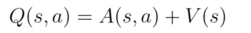
Remember that Q-values correspond to how good it is to be at that state and taking an action at that state Q(s,a).
So we can decompose Q(s,a) as the sum of:
- V(s): the value of being at that state
- A(s,a): the advantage of taking that action at that state (how much better is to take this action versus all other possible actions at that state).
With DDQN, we want to separate the estimator of these two elements, using two new streams:
- one that estimates the state value V(s)
- one that estimates the advantage for each action A(s,a)
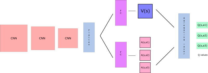
And then we combine these two streams through a special aggregation layer to get an estimate of Q(s,a).
Wait? But why do we need to calculate these two elements separately if then we combine them?
By decoupling the estimation, intuitively our DDQN can learn which states are (or are not) valuable without having to learn the effect of each action at each state (since it’s also calculating V(s)).
With our normal DQN, we need to calculate the value of each action at that state. But what’s the point if the value of the state is bad? What’s the point to calculate all actions at one state when all these actions lead to death?
As a consequence, by decoupling we’re able to calculate V(s). This is particularly useful for states where their actions do not affect the environment in a relevant way. In this case, it’s unnecessary to calculate the value of each action. For instance, moving right or left only matters if there is a risk of collision. And, in most states, the choice of the action has no effect on what happens.
It will be clearer if we take the example in the paper Dueling Network Architectures for Deep Reinforcement Learning.
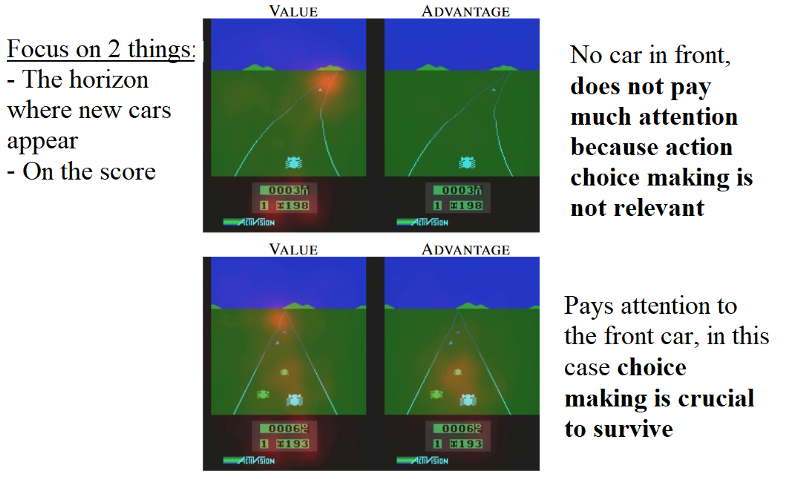
We see that the value network streams pays attention (the orange blur) to the road, and in particular to the horizon where the cars are spawned. It also pays attention to the score.
On the other hand, the advantage stream in the first frame on the right does not pay much attention to the road, because there are no cars in front (so the action choice is practically irrelevant). But, in the second frame it pays attention, as there is a car immediately in front of it, and making a choice of action is crucial and very relevant.
Concerning the aggregation layer, we want to generate the q values for each action at that state. We might be tempted to combine the streams as follows:
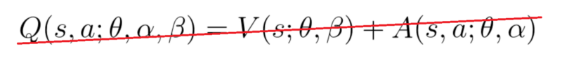
But if we do that, we’ll fall into the issue of identifiability, that is — given Q(s,a) we’re unable to find A(s,a) and V(s).
And not being able to find V(s) and A(s,a) given Q(s,a) will be a problem for our back propagation. To avoid this problem, we can force our advantage function estimator to have 0 advantage at the chosen action.
To do that, we subtract the average advantage of all actions possible of the state.
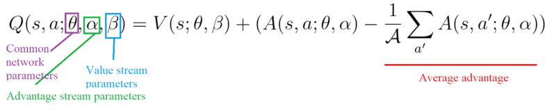
Therefore, this architecture helps us accelerate the training. We can calculate the value of a state without calculating the Q(s,a) for each action at that state. And it can help us find much more reliable Q values for each action by decoupling the estimation between two streams.
Implementation
The only thing to do is to modify the DQN architecture by adding these new streams:
Prioritized Experience Replay
Theory
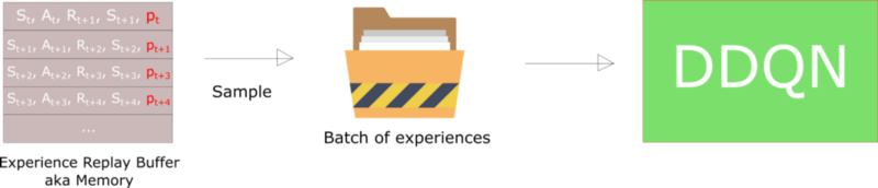
Prioritized Experience Replay (PER) was introduced in 2015 by Tom Schaul. The idea is that some experiences may be more important than others for our training, but might occur less frequently.
Because we sample the batch uniformly (selecting the experiences randomly) these rich experiences that occur rarely have practically no chance to be selected.
That’s why, with PER, we try to change the sampling distribution by using a criterion to define the priority of each tuple of experience.
We want to take in priority experience where there is a big difference between our prediction and the TD target, since it means that we have a lot to learn about it.
We use the absolute value of the magnitude of our TD error:
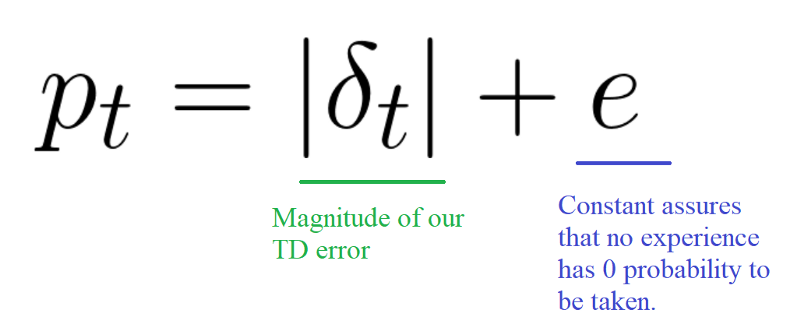
And we put that priority in the experience of each replay buffer.
But we can’t just do greedy prioritization, because it will lead to always training the same experiences (that have big priority), and thus over-fitting.
So we introduce stochastic prioritization, which generates the probability of being chosen for a replay.
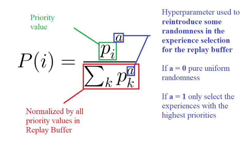
As consequence, during each time step, we will get a batch of samples with this probability distribution and train our network on it.
But, we still have a problem here. Remember that with normal Experience Replay, we use a stochastic update rule. As a consequence, the way we sample the experiences must match the underlying distribution they came from.
When we do have normal experience, we select our experiences in a normal distribution — simply put, we select our experiences randomly. There is no bias, because each experience has the same chance to be taken, so we can update our weights normally.
But, because we use priority sampling, purely random sampling is abandoned. As a consequence, we introduce bias toward high-priority samples (more chances to be selected).
And, if we update our weights normally, we take have a risk of over-fitting. Samples that have high priority are likely to be used for training many times in comparison with low priority experiences (= bias). As a consequence, we’ll update our weights with only a small portion of experiences that we consider to be really interesting.
To correct this bias, we use importance sampling weights (IS) that will adjust the updating by reducing the weights of the often seen samples.
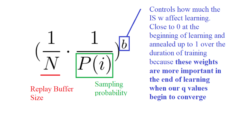
The weights corresponding to high-priority samples have very little adjustment (because the network will see these experiences many times), whereas those corresponding to low-priority samples will have a full update.
The role of b is to control how much these importance sampling weights affect learning. In practice, the b parameter is annealed up to 1 over the duration of training, because these weights are more important in the end of learning when our q values begin to converge. The unbiased nature of updates is most important near convergence, as explained in this article.
Implementation
This time, the implementation will be a little bit fancier.
First of all, we can’t just implement PER by sorting all the Experience Replay Buffers according to their priorities. This will not be efficient at all due to O(nlogn) for insertion and O(n) for sampling.
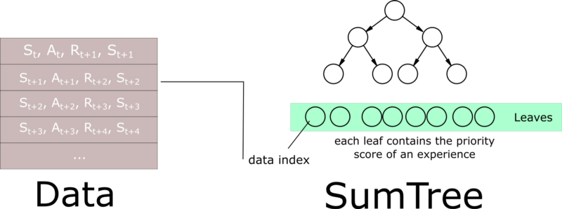
As explained in this really good article, we need to use another data structure instead of sorting an array — an unsorted sumtree.
A sumtree is a Binary Tree, that is a tree with only a maximum of two children for each node. The leaves (deepest nodes) contain the priority values, and a data array that points to leaves contains the experiences.
Updating the tree and sampling will be really efficient (O(log n)).
Then, we create a memory object that will contain our sumtree and data.
Next, to sample a minibatch of size k, the range [0, total_priority] will be divided into k ranges. A value is uniformly sampled from each range.
Finally, the transitions (experiences) that correspond to each of these sampled values are retrieved from the sumtree.
It will be much clearer when we dive on the complete details in the notebook.
Doom Deathmatch agent
This agent is a Dueling Double Deep Q Learning with PER and fixed q-targets.
We made a video tutorial of the implementation:
The notebook is here
That’s all! You’ve just created an smarter agent that learns to play Doom. Awesome! Remember that if you want to have an agent with really good performance, you need many more GPU hours (about two days of training)!
However, with only 2–3 hours of training on CPU (yes CPU), our agent understood that they needed to kill enemies before being able to move forward. If they move forward without killing enemies, they will be killed before getting the vest.
Don’t forget to implement each part of the code by yourself. It’s really important to try to modify the code I gave you. Try to add epochs, change the architecture, add fixed Q-values, change the learning rate, use a harder environment…and so on. Experiment, have fun!
Remember that this was a big article, so be sure to really understand why we use these new strategies, how they work, and the advantages of using them.
In the next article, we’ll learn about an awesome hybrid method between value-based and policy-based reinforcement learning algorithms. This is a baseline for the state of the art’s algorithms: Advantage Actor Critic (A2C). You’ll implement an agent that learns to play Outrun !
If you liked my article, please click the ? below as many time as you liked the article so other people will see this here on Medium. And don’t forget to follow me!
If you have any thoughts, comments, questions, feel free to comment below or send me an email: hello@simoninithomas.com, or tweet me @ThomasSimonini.


Keep learning, stay awesome!
Deep Reinforcement Learning Course with Tensorflow ?️
? Syllabus
? Video version
Part 1: An introduction to Reinforcement Learning
Part 2: Diving deeper into Reinforcement Learning with Q-Learning
Part 3: An introduction to Deep Q-Learning: let’s play Doom
Part 4: An introduction to Policy Gradients with Doom and Cartpole
Part 5: An intro to Advantage Actor Critic methods: let’s play Sonic the Hedgehog!
Part 6: Proximal Policy Optimization (PPO) with Sonic the Hedgehog 2 and 3