By Patryk Miziuła
This article was written by Piotr Migdał, Rafał Jakubanis and myself. In the previous post, they gave you an overview of the differences between Keras and PyTorch, aiming to help you pick the framework that’s better suited to your needs.
Now, it’s time for a trial by combat.
We’re going to pit Keras and PyTorch against each other, showing their strengths and weaknesses in action. We present a real problem, a matter of life-and-death: distinguishing Aliens from Predators!
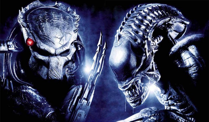 Image taken from our dataset. Both Predator and Alien are deeply interested in AI.
We’ll perform image classification, one of the computer vision tasks deep learning shines at. As training from scratch is unfeasible in most cases (as it is very data hungry), we’ll perform transfer learning using ResNet-50 pre-trained on ImageNet. We’ll get as practical as possible, to show both the conceptual differences and conventions.
At the same time we’ll keep the code fairly minimal, to make it clear and easy to read and reuse. See notebooks on GitHub, Kaggle kernels or Neptune versions with fancy charts.
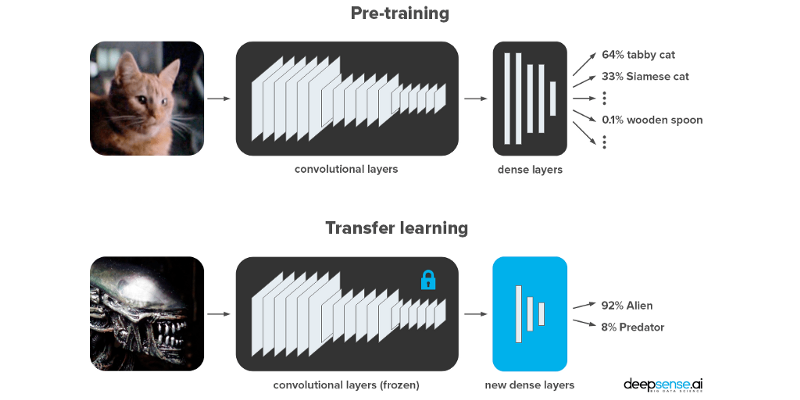
Wait, what’s transfer learning? And why ResNet-50?
In practice, very few people train an entire Convolutional Network from scratch (with random initialization), because it is relatively rare to have a dataset of sufficient size. Instead, it is common to pretrain a ConvNet on a very large dataset (e.g. ImageNet, which contains 1.2 million images with 1000 categories), and then use the ConvNet either as an initialization or a fixed feature extractor for the task of interest. — Andrej Karpathy, Transfer Learning — CS231n Convolutional Neural Networks for Visual Recognition
Transfer learning is a process of making tiny adjustments to a network trained on a given task to perform another, similar task.
In our case we’re working with the ResNet-50 model trained to classify images from the ImageNet dataset. It is enough to learn a lot of textures and patterns that may be useful in other visual tasks, even as alien as this Alien vs. Predator case. That way, we’ll use much less computing power to achieve much better results.
In our case we’re going to do it the simplest possible way:
- keep the pre-trained convolutional layers (so-called feature extractor), with their weights frozen, and
- remove the original dense layers, and replace them with brand-new dense layers we will use for training.
So, which network should we choose as the feature extractor?
ResNet-50 is a popular model for ImageNet image classification (AlexNet, VGG, GoogLeNet, Inception, Xception are other popular models). It is a 50-layer deep neural network architecture based on residual connections, which are connections that add modifications with each layer, rather than completely changing the signal.
ResNet was the state-of-the-art on ImageNet in 2015. Since then, newer architectures with higher scores on ImageNet have been invented. However, they are not necessarily better at generalizing to other datasets (see the Do Better ImageNet Models Transfer Better? arXiv paper).
Ok, it’s time to dive into the code.
Let the match begin!
We’ll set up our Alien vs. Predator challenge in seven steps:
- Prepare the dataset
- Import dependencies
- Create data generators
- Create the network
- Train the model
- Save and load the model
- Make predictions on sample test images
We’re supplementing this blog post with Python code in Jupyter Notebooks (Keras-ResNet50.ipynb, PyTorch-ResNet50.ipynb). This environment is more convenient for prototyping than bare scripts, as we can execute it cell by cell and peak into the output.
All right, let’s go!
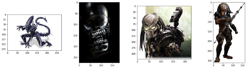
0. Prepare the dataset
We created a dataset by performing a Google Search with the words “alien” and “predator”. We saved JPG thumbnails (around 250×250 pixels) and manually filtered the results. Here are some examples:
We split our data into two parts:
- Training data (347 samples per class) — used for training the network.
- Validation data (100 samples per class) — not used during the training, but needed in order to check the performance of the model on previously unseen data.
Keras requires the datasets to be organized in folders in the following way:
If you want to see the process of organizing data into directories, check out the data_prep.ipynb file. You can download the dataset from Kaggle.
1. Import dependencies
First, the technicalities. We’re assuming that you have Python 3.5+, Keras 2.2.2 (with TensorFlow 1.10.1 backend) and PyTorch 0.4.1. Check out the requirements.txt file in the repo.
So, first, we need to import the required modules. We’ll separate the code in Keras, PyTorch and common (one required in both).
We can check the frameworks’ versions by typing keras.__version__ and torch.__version__, respectively.
2. Create data generators
Normally, the images can’t all be loaded at once, as doing so would be too much for the memory to handle. At the same time, we want to benefit from the GPU’s performance boost by processing a few images at once. So we load images in batches (e.g. 32 images at once) using data generators. Each pass through the whole dataset is called an epoch.
We also use data generators for preprocessing: we resize and normalize images to make them as ResNet-50 likes them (224 x 224 px, with scaled color channels). And last but not least, we use data generators to randomly perturb images on the fly:
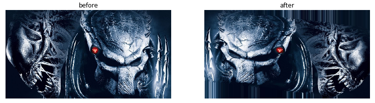
Performing such changes is called data augmentation. We’ll use it to show a neural network which kinds of transformations don’t matter. Or, to put it another way, we’ll train on a potentially infinite dataset by generating new images based on the original dataset.
Almost all visual tasks benefit, to varying degrees, from data augmentation for training. For more info about data augmentation, see as applied to plankton photos or how to use it in Keras. In our case, we randomly shear, zoom and horizontally flip our aliens and predators.
Here we create generators that:
- load data from folders,
- normalize data (both train and validation), and
- augment data (train only).
In Keras, you get built-in augmentations and preprocess_input method normalizing images put to ResNet-50, but you have no control over their order. In PyTorch, you have to normalize images manually, but you can arrange augmentations in any way you like.
There are also other nuances: for example, Keras by default fills the rest of the augmented image with the border pixels (as you can see in the picture above) whereas PyTorch leaves it black. Whenever one framework deals with your task much better than the other, take a closer look to see if they perform preprocessing identically; we bet they don’t.
3. Create the network
The next step is to import a pre-trained ResNet-50 model, which is a breeze in both cases. We’ll freeze all the ResNet-50’s convolutional layers, and only train the last two fully connected (dense) layers. As our classification task has only 2 classes (compared to 1000 classes of ImageNet), we need to adjust the last layer.
Here we:
- load pre-trained network, cut off its head and freeze its weights,
- add custom dense layers (we pick 128 neurons for the hidden layer), and
- set the optimizer and loss function.
We load the ResNet-50 from both Keras and PyTorch without any effort. They also offer many other well-known pre-trained architectures: see Keras’ model zoo and PyTorch’s model zoo. So, what are the differences?
In Keras we may import only the feature-extracting layers, without loading extraneous data (include_top=False). We then create a model in a functional way, using the base model’s inputs and outputs. Then we use model.compile(...) to bake into it the loss function, optimizer and other metrics.
In PyTorch, the model is a Python object. In the case of models.resnet50, dense layers are stored in model.fc attribute. We’ll overwrite them. The loss function and optimizers are separate objects. For the optimizer, we need to explicitly pass a list of parameters we want it to update.
In PyTorch, we should explicitly specify what we want to load to the GPU using .to(device) method. We have to write it each time we intend to put an object on the GPU, if available. Well…
 Frame from ‘AVP: Alien vs. Predator’: Predators’ wrist computer. We’re pretty sure Predator could use it to compute logsoftmax.
Layer freezing works in a similar way. However, in The Batch Normalization layer of Keras is broken (as of the current version; thx Przemysław Pobrotyn for bringing this issue), you’ll see that some layers get modified anyway, even with trainable=False.
Keras and PyTorch deal with log-loss in a different way.
In Keras, a network predicts probabilities (has a built-in softmax function), and its built-in cost functions assume they work with probabilities.
In PyTorch we have more freedom, but the preferred way is to return logits. This is done for numerical reasons, performing softmax then log-loss means doing unnecessary log(exp(x)) operations. So, instead of using softmax, we use LogSoftmax (and NLLLoss) or combine them into one nn.CrossEntropyLoss loss function.
4. Train the model
OK, ResNet is loaded, so let’s get ready to space rumble!
 Frame from ‘AVP: Alien vs. Predator’: the Predators’ Mother Ship. Yes, we’ve heard that there are no rumbles in space, but nothing is impossible for Aliens and Predators.
Now, we’ll proceed to the most important step — model training. We need to pass data, calculate the loss function and modify network weights accordingly. While we already had some differences between Keras and PyTorch in data augmentation, the length of code was similar. For training… the difference is massive. Let’s see how it works!
Here we:
- train the model, and
- measure the loss function (log-loss) and accuracy for both training and validation sets.
In Keras, the model.fit_generator performs the training… and that’s it! Training in Keras is just that convenient. And as you can find in the notebook, Keras also gives us a progress bar and a timing function for free. But if you want to do anything nonstandard, then the pain begins…
PyTorch is on the other pole. Everything is explicit here. You need more lines to construct the basic training, but you can freely change and customize all you want.
 Predator’s shuriken returning to its owner automatically. Would you prefer to implement its tracking ability in Keras or PyTorch?
Let’s shift gears and dissect the PyTorch training code. We have nested loops, iterating over:
- epochs,
- training and validation phases, and
- batches.
The epoch loop does nothing but repeat the code inside. The training and validation phases are done for three reasons:
- Some special layers, like batch normalization (present in ResNet-50) and dropout (absent in ResNet-50), work differently during training and validation. We set their behavior by
model.train()andmodel.eval(), respectively. - We use different images for training and for validation, of course.
- The most important and least surprising thing: we train the network during training only. The magic commands
optimizer.zero_grad(),loss.backward()andoptimizer.step()(in this order) do the job. If you know what backpropagation is, you appreciate their elegance.
We then take care of computing the epoch losses and prints ourselves.
5. Save and load the model
Saving
Once our network is trained, often with high computational and time costs, it’s good to keep it for later. Broadly, there are two types of savings:
- saving the whole model architecture and trained weights (and the optimizer state) to a file, and
- saving the trained weights to a file (keeping the model architecture in the code).
It’s up to you which way you choose.
Here we:
- save the model.
One line of code is enough in both frameworks. In Keras you can either save everything to a HDF5 file or save the weights to HDF5 and the architecture to a readable JSON file. By the way: you can then load the model and run it in the browser.
 Frame from ‘Alien: Resurrection’: Alien is evolving, just like PyTorch.
Currently, PyTorch creators recommend saving the weights only. They discourage saving the whole model because the API is still evolving.
Loading
Loading models is as simple as saving. You should just remember which saving method you chose and the file paths.
Here we:
- load the model.
In Keras we can load a model from a JSON file, instead of creating it in Python (at least when we don’t use custom layers). This kind of serialization makes it convenient for transferring models.
PyTorch can use any Python code. So pretty much we have to re-create a model in Python.
Loading model weights is similar in both frameworks.
6. Make predictions on sample test images
All right, it’s finally time to make some predictions! To fairly check the quality of our solution, we’ll ask the model to predict the type of monsters from images not used for training. We can use the validation set, or any other image.
Here we:
- load and preprocess test images,
- predict image categories, and
- show images and predictions.
Prediction, like training, works in batches (here we use a batch of 3; though we could surely also use a batch of 1).
In both Keras and PyTorch we need to load and preprocess the data. A rookie mistake is to forget about the preprocessing step (including color scaling). It is likely to work, but will result in worse predictions (since it effectively sees the same shapes but with different colors and contrasts).
In PyTorch there are two more steps, as we need to:
- convert logits to probabilities, and
- transfer data to the CPU and convert to NumPy (fortunately, the error messages are fairly clear when we forget this step).
And this is what we get:

It works!
And how about other images? If you can’t come up with anything (or anyone) else, try using photos of your co-workers. ?
Conclusion
As you can see, Keras and PyTorch differ significantly in terms of how standard deep learning models are defined, modified, trained, evaluated, and exported. For some parts it’s purely about different API conventions, while for others fundamental differences between levels of abstraction are involved.
Keras operates on a much higher level of abstraction. It is much more plug&play, and typically more succinct, but at the cost of flexibility.
PyTorch provides more explicit and detailed code. In most cases it means debuggable and flexible code, with only small overhead. Yet, training is way-more verbose in PyTorch. It hurts, but at times provides a lot of flexibility.
Transfer learning is a big topic. Try tweaking your parameters (e.g. dense layers, optimizer, learning rate, augmentation) or choose a different network architecture.
Have you tried transfer learning for image recognition? Consider the list below for some inspiration:
- Chihuahua vs. muffin, sheepdog vs. mop, shrew vs. kiwi (already serves as an interesting benchmark for computer vision)
- Original images vs. photoshopped ones
- Artichoke vs. broccoli vs. cauliflower
- Zerg vs. Protoss vs. Orc vs. Elf
- Meme or not meme
- Is it a picture of a bird?
- Is it huggable?
Pick Keras or PyTorch, choose a dataset, and let us know how it went in the comments section below ?
By the way, in November we are running a series of hands-on training where you can learn more about Keras and PyTorch. Piotr Migdał and I will lead some of the sessions so feel free to check it out.