
By Neil Kakkar
Meet Mason. He's an average American 40-year-old: 5 foot 10 inches tall and earning $47,000 per year before tax.
How often would you expect to meet someone who earns 10x as much as Mason?
And now, how often would you expect to meet someone who is 10x as tall as Mason?
Your answers to the two questions above are different, because the distribution of data is different. In some cases, 10x above average is common. While in others, it's not common at all.
So what are normal distributions?
Today, we're interested in normal distributions. They are represented by a bell curve: they have a peak in the middle that tapers towards each edge. A lot of things follow this distribution, like your height, weight, and IQ.
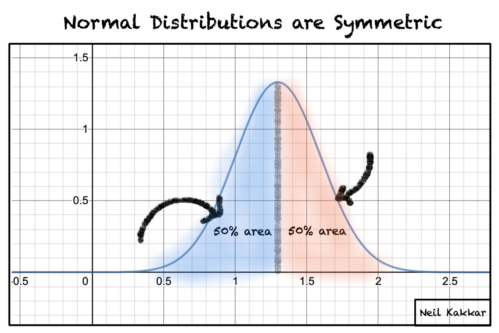
This distribution is exciting because it's symmetric – which makes it easy to work with. You can reduce lots of complicated mathematics down to a few rules of thumb, because you don't need to worry about weird edge cases.
For example, the peak always divides the distribution in half. There's equal mass before and after the peak.
Another important property is that we don't need a lot of information to describe a normal distribution.
Indeed, we only need two things:
- The mean. Most people just call this "the average." It's what you get if you add up the value of all your observations, then divide that number by the number of observations. For example, the average of these three numbers:
1, 2, 3 = (1 + 2 + 3) / 3 = 2 - And the standard deviation. This tells you how rare an observation would be. Most observations fall within one standard deviation of the mean. Fewer observations are two standard deviations from the mean. And even fewer are three standard deviations away (or further).
Together, the mean and the standard deviation make up everything you need to know about a distribution.
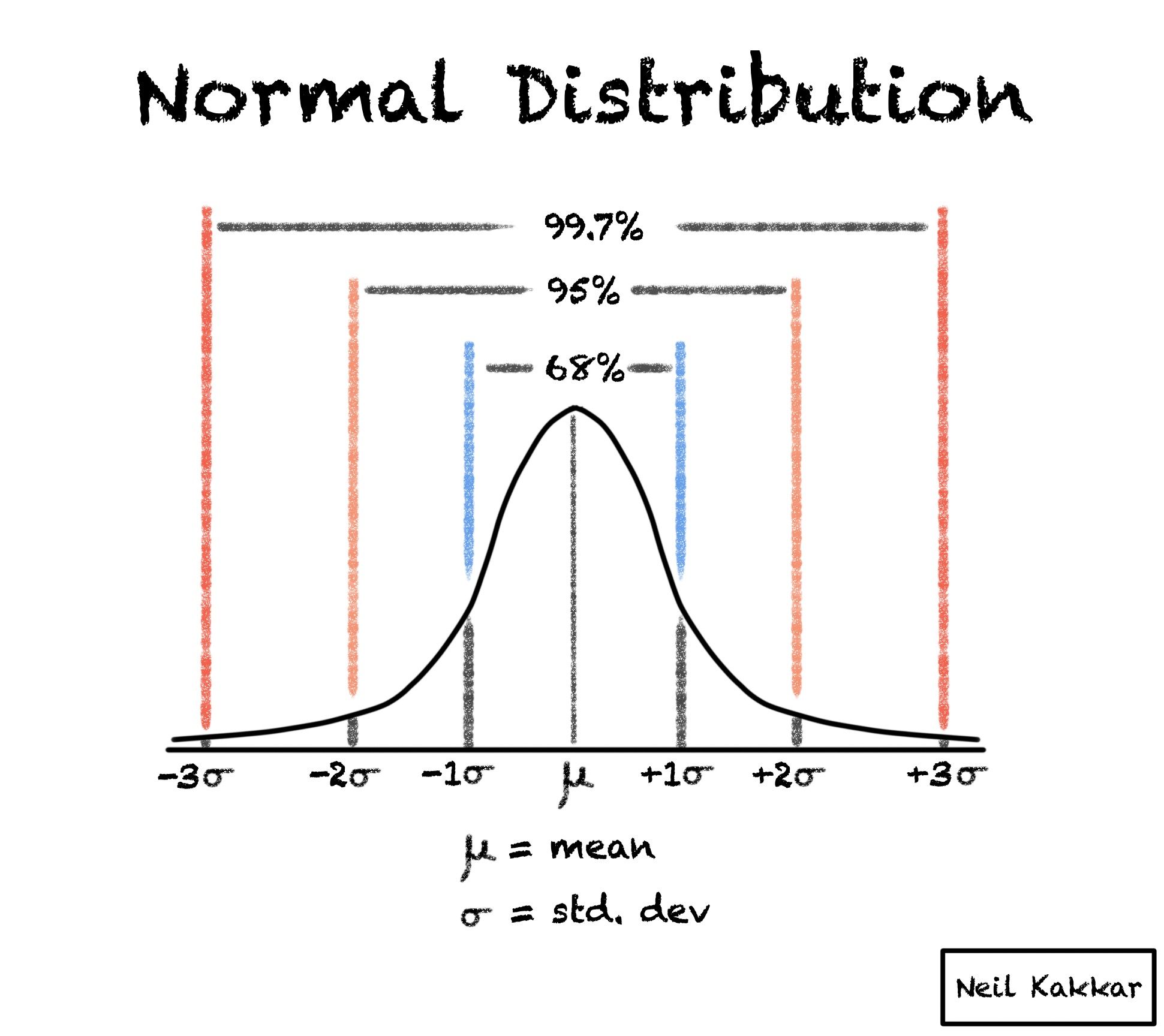
The 68-95-99 rule
The 68-95-99 rule is based on the mean and standard deviation. It says:
68% of the population is within 1 standard deviation of the mean.
95% of the population is within 2 standard deviation of the mean.
99.7% of the population is within 3 standard deviation of the mean.
How to calculate normal distributions
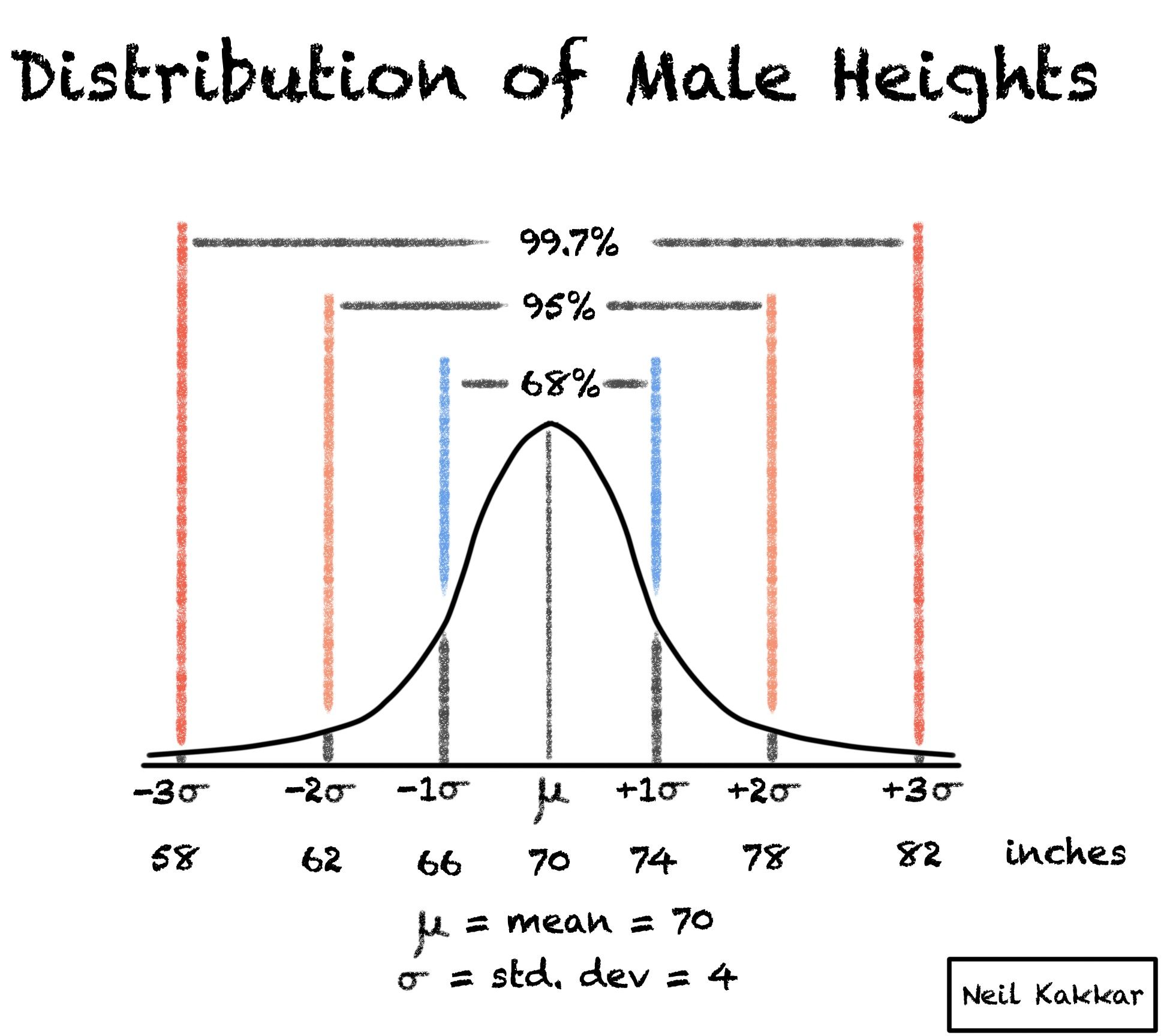
To continue our example, the average American male height is 5 feet 10 inches, with a standard deviation of 4 inches. This means:
Now for the fun part: Let's apply what we've just learned.
What's the chance of seeing someone with a height between between 5 feet 10 inches and 6 feet 2 inches? (That is, between 70 and 74 inches.)
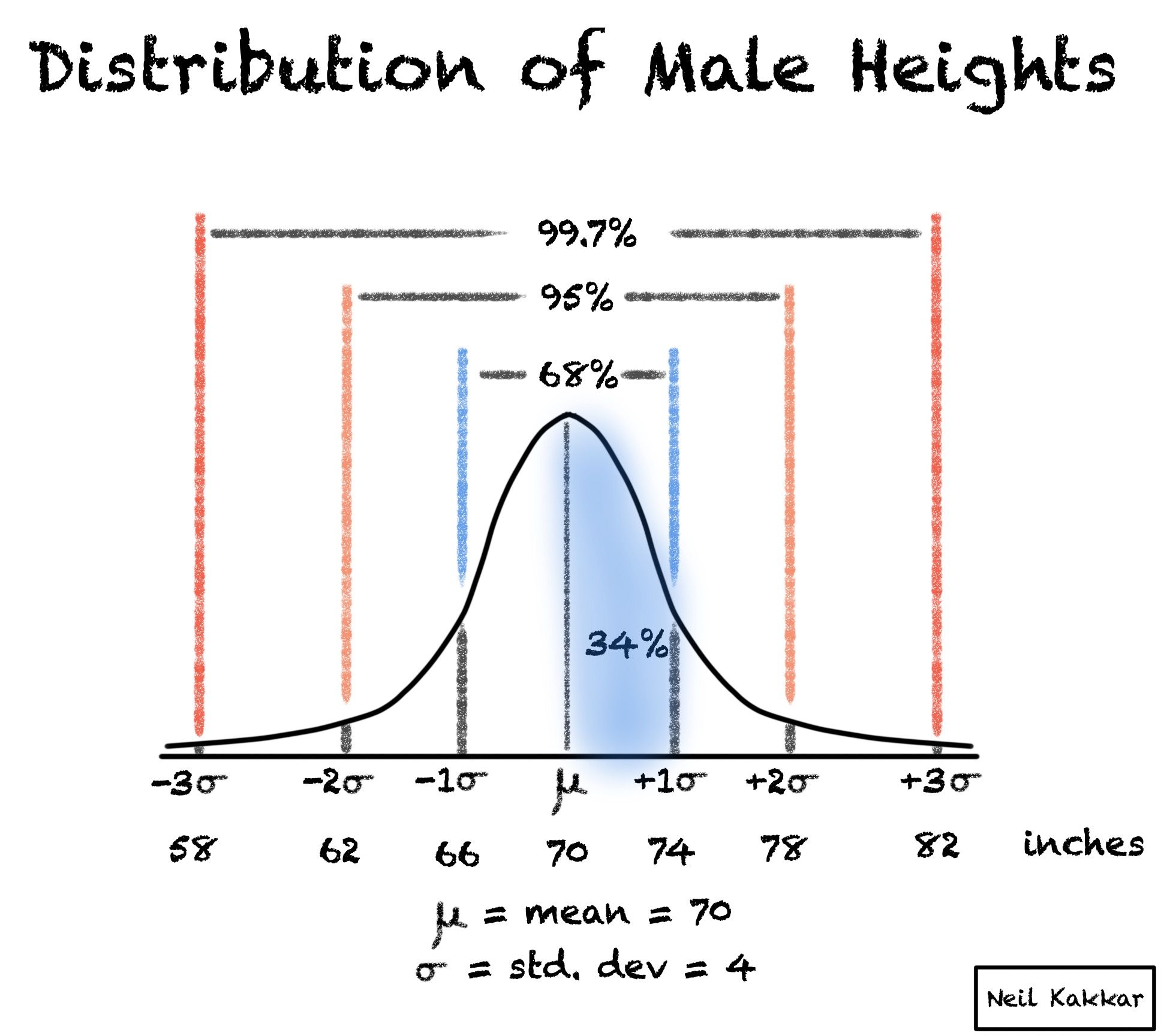
It's 34%! We leverage both the properties: the distribution is symmetric, which means chances for (66-70) inches and (70-74) inches are both 68/2 = 34%.
Let's try a tougher one. What's the chance of seeing someone with a height between 62 and 66 inches?
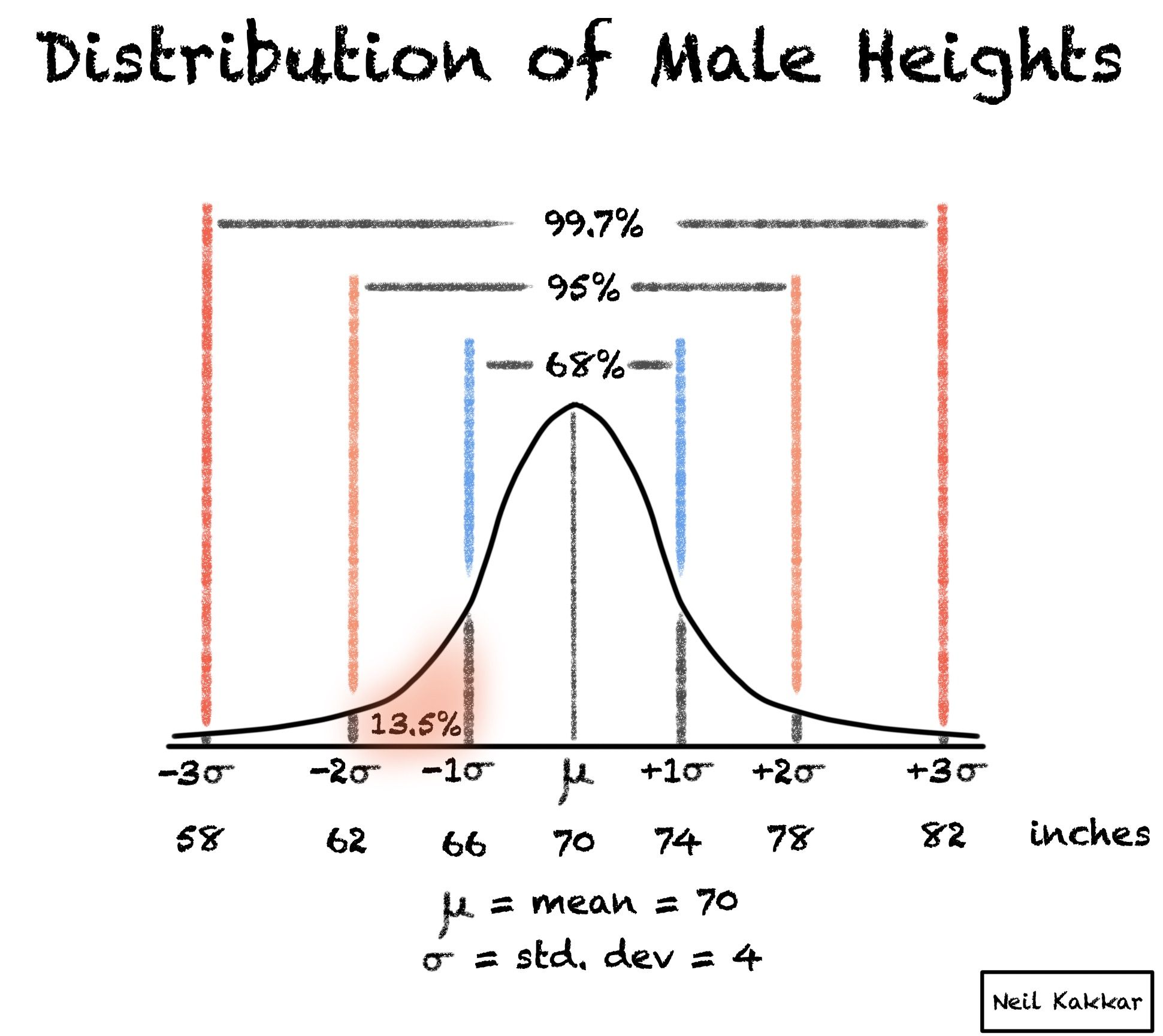
It's (95-68)/2 = 13.5%. Both outer edges have the same %.
And now your final (and hardest test): What's the chance of seeing someone with a height greater than 82 inches?
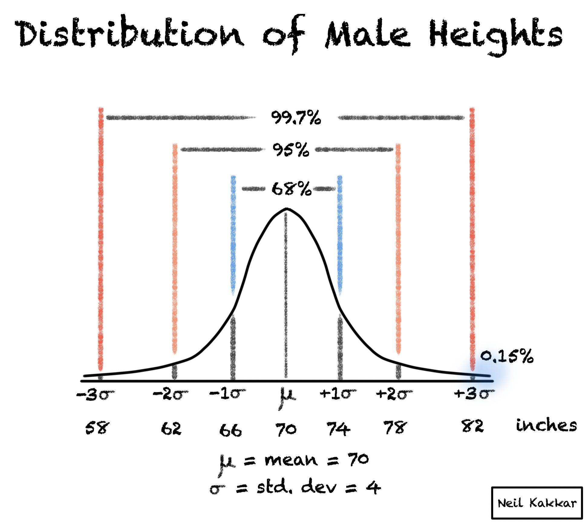
Here, we use also the final property: everything must sum to 100%. So the outer edges (that is, heights below 58 and heights above 82) together make (100% - 99.7%) = 0.3%.
Remember, you can apply this on any normal distribution. Try doing the same for female heights: the mean is 65 inches, and standard deviation is 3.5 inches.
So, the chance of seeing someone with a height between 65 and 68.5 inches would be: ___.
...
...
34%! It's exactly the same as our first example. It's +1 standard deviation.
Conclusion
Knowing this rule makes it very easy to calibrate your senses. Since all we need to describe any normal distribution is the mean and standard deviation, this rule holds for every normal distribution in the world!
The challenging part, indeed, is figuring out whether the distribution is normal or not.
Want to learn more about calibrating your senses and thinking critically? Check out Bayes Theorem: A Framework for Critical Thinking.