
By Michelle Jones
What is a p-value?
If your experiment needs statistics, you ought to have done a better experiment. — Ernest Rutherford
The use of p-values in research is very common. Peer reviewed journal articles are chock-full of them. It seems like every scientist and their salivating dog uses them.
Okay, without looking up the answer:
what is the definition of a p-value?
Be honest, I won’t tell anyone your answer. I promise. It’s our secret. We’ll keep coming back to this question over my next few posts.
We’re starting our journey with Pearson.
Karl Pearson
In 1900, Karl Pearson published his paper that discussed the concept of p-values. Most of the paper is worked examples of the form that we know as the chi-squared test. Thus, the focus of the paper is on frequencies of counts, and the degree to which observed counts differ (in Pearson’s term, deviate) from expected counts. In his statistical terms, each deviation (n) is an error.
His definition of P was as follows:
the probability of a complex system of n errors occurring with a frequency as great or greater than that of the observed system (p.158)
In other words, given the expected counts, how probable are our observed counts and counts that are even more different?
Two main types of chi-squared tests
There is one key point to note about Fisher’s chi-squared test. Yes, his method determines whether observed counts differ from the expected counts. However, he directly compared observed counts to their expected counts based on a pre-determined, underlying distribution. This is a goodness-of-fit test. The sorts of questions he was asking were:
- does this set of results of dice rolls follow a binomial distribution?
- does this set of petal counts from 222 buttercups fit a specific skew curve?
This is completely different to how we normally use a chi-squared test, where we compare two groups, rather than one group to a predefined distribution:
- do cases and controls (e.g. smokers/non-smokers) significantly differ on disease incidence (e.g. lung cancer)?
- do men and women vote for the same political candidates?
In our normal case, the expected counts (and therefore distribution) are directly derived from the contingency table margins. In this second method, we are performing the chi-square test of independence. (There’s another type of chi-squared test that basically uses the same analysis as this one, but that’s a technicality we will be ignoring.)
Back to the chi squared goodness-of-fit test.
Dice rolling
Let’s work through Pearson’s first example using R. Base R is sufficient for this. We’ll use R to work out the chi-squared value (χ²) for ourselves. Finally, we’ll sum the theoretical and observed counts as a check that the numbers are what we expect from the table in the paper.
Description of experiment
The data arise from an experiment where twelve dice were rolled 26,306 times. In each roll, the number of dice with a 5 or 6 showing were counted. (I imagine it was some poor graduate student who drew the short straw.)
With 12 dice, the range of possible numbers on each throw is from zero (no die had a 5 or 6 showing) to twelve (all dice had a 5 or 6 showing).
Binomial distribution
The values for rolled dice follow a binomial distribution. We use this distribution for count data. For those interested in the relationship between the binomial distribution and the chi-squared test, this is an accessible explanation.
The expected values for each possible value in the range 0 through 12 can be calculated using the dbinom function in R. For example, the probability of obtaining zero dice showing a 5 or 6 when 12 dice are rolled is
dbinom(0,12,1/3)[1] 0.007707347
We multiply the probability by the total number of trials to get the expected count for no 5s and no 6s across the 26,306 trials
dbinom(0,12,1/3)*26306[1] 202.7495
Which we round up to 203. We can repeat this process for the values 1 through 12. However, when we reach 12 we get the following problem.
dbinom(12,12,1/3)[1] 1.881676e-06
dbinom(12,12,1/3)*26306[1] 0.04949938
Our probability and associated count are extremely close to 0. More on this below.
Create the data.frame
We’ll construct the data.frame as we read in the values.
PearsonChiSquare <- data.frame(Face5or6=c(0,1,2,3,4,5,6,7,8,9,10,11,12), Theoretical=c(203,1217,3345,5576,6273,5018,2927,1254,392,87,13,1,0), Observed=c(185,1149,3265,5475,6114,5194,3067,1331,403,105,14,4,0))
Back to the problem with our data, that will only show when we perform the chi-squared test. Notice the 0 theoretical and expected counts for all 12 dice showing 5 or 6? The chi-squared test will not give us a result when there is division by 0.
What can we do? The easiest method to deal with this problem is to remove the last row of the data.frame. In our case, this is exactly the same as combining the 11 and 12 categories (the normal method when cell counts are very small). Our trial count is still the same. Our underlying probabilities sum almost to 1. We will do a little correction for that.
We drop the row where the theoretical value is 0. I could have addressed this problem by simply not reading in the 0 values. However, dropping a data.frame row based on a value is a common task in R. This code can be generalised to any instance where you need to drop one or more rows on the basis of a specific value of a variable.
#as group of 12 has 0 theoretical and 0 observed counts, drop this observationPearsonChiSquare <- PearsonChiSquare[!(PearsonChiSquare$Theoretical==0),]
Now we construct our column of theoretical probabilities based on the remaining data. Remember, the probability of having twelve dice with 5s or 6s was very small, but was not zero. Thus, the probabilities calculated for each row of our remaining data will slightly differ from the probabilities that Pearson was using.
PearsonChiSquare$probs <- with(PearsonChiSquare, Theoretical/sum(Theoretical))
Why do we need to create a column of probabilities? Because we are doing a goodness-of-fit test. We are comparing each observed count to the probability of that count, assuming a binomial distribution.
Chi-squared test
Now we are ready to do our chi-squared test. The output is shown below the command.
chisq.test(x=PearsonChiSquare$Observed, p=PearsonChiSquare$probs)
Chi-squared test for given probabilities
data: PearsonChiSquare$ObservedX-squared = 43.876, df = 11, p-value = 7.641e-06
The function automatically calculates the number of degrees of freedom (df) from our data. The calculation for the number of df in the chi-squared test is very easy. It is (rows -1) x (columns-1).
We have 12 categories (range 0 to 11 = 12 categories). We have two columns (observed counts, binomial probabilities). Our df are therefore (12–1) x (2–1) = 11 x 1 = 11.
How did we do for the χ2 value? Especially as we removed one row of data?
Pearson calculated χ2=43.87241. We got really close! He calculated P=0.000016. He argued that his result gave 62,499 to 1 against the observed values arising from a binomial distribution. Putting our result into decimal notation, we got P=0.0000076.
Our p-value is very small. We reject the null hypothesis that our observed results arise from a binomial distribution.
What is causing the difference?
The reason for this is the positive bias towards rolling a 5 or 6 (except in the extreme case of all 5s or 6s). We can duplicate this bias by calculating the deviations of the observed values from the theoretical values, duplicating more of Pearson’s work.
The code below performs this calculation and then writes the values to the console.
PearsonChiSquare$Deviation <- with(PearsonChiSquare,Observed-Theoretical)
PearsonChiSquare[, c("Face5or6","Deviation")]
Face5or6 Deviation1 0 -182 1 -683 2 -804 3 -1015 4 -1596 5 1767 6 1408 7 779 8 1110 9 1811 10 112 11 3
As you can see, the observed counts for trials where five or fewer dice showed a 5 or 6 are lower than expected (these are all negative values). Conversely, observed counts for trials where six or more dice showed a 5 or 6 are higher than expected (these are all positive values).
Interpreting the p-value
Paraphrasing, Pearson said that the the p-value is the probability of results that are as improbable or more improbable than the one encountered. Our p-value is the probability of getting our χ2 value and any larger χ2 value.
Why isn’t the p-value related only to the counts that we fitted? The p-value arises from a cumulative density function. The probability of obtaining our exact results, or any specified counts, is very close to 0. For the chi-squared statistic, we are evaluating the integral where our χ2 value is the lower bound. For the very interested, here is a description of the maths.
Visualizing chi-squared p-values in R
Our chi-squared distribution
We can visualise the chi-squared distribution in R. Let’s draw the probability distribution for the chi-squared distribution when there are 11 degrees of freedom. Remember, our test had 11 degrees of freedom. As you can see, I’m using my favourite package for this.
library("ggplot2")ggplot(data.frame(x=c(0,50)), aes(x=x))+ stat_function(fun=dchisq, args=list(df=11))+ labs(title="Chi-squared probability distribution for 11 df", x="Chi-squared value", y="Probability")
This produces the following graph.
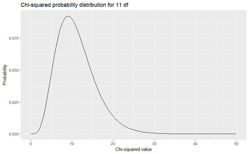
We read the probabilities associated with the χ2 values from right to left. As you can see from the graph, the probability of getting any χ2 value larger than 40 is extremely small. We know it is below 0.000 because the line is flat at that point. Probabilities can get very small, but they cannot reach zero.
Pearson’s chi-squared distribution
What about if we had Pearson’s original 12 degrees of freedom, because we didn’t drop that group (and assume we fudged about the 0 problem)? Let’s overlay the probability distributions for 12 degrees of freedom over the distribution we already plotted.
ggplot(data.frame(x=c(0,50)), aes(x=x))+ stat_function(fun=dchisq, args=list(df=11), aes(colour="11 df"))+ stat_function(fun=dchisq, args=list(df=12), aes(colour="12 df"))+ scale_colour_manual(name="", values=c("black","blue"))+ labs(title="Chi-squared probability distribution for 11 and 12 df", x="Chi-squared value", y="Probability")
Which produces the graph:
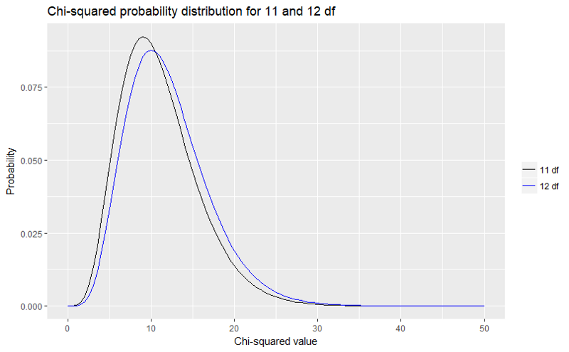
We can see that the difference between our χ2 value and Pearson’s _χ2 value is negligible, considered against the relevant χ_2 probability distribution.
In practical terms, the χ2 value has to be quite small in order to accept the null hypothesis. The null hypothesis, in this case, is that the observed data arise from a binomial distribution.
Showing the rejection area for specific p-values
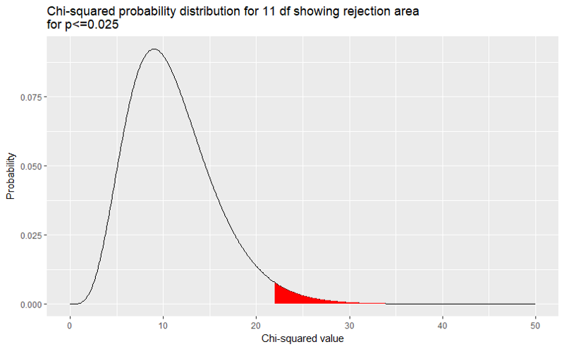
We can show how the p-value changes as the χ2 value is decreased. This also shows how the χ2 acts as the lower bound on the rejection area. If we want to reject at P ≤ 0.025, we can show the rejection area on the graph.
RejectionArea <- data.frame(x=seq(0,50,0.1))RejectionArea$y <- dchisq(RejectionArea$x,11)
library(ggplot2)ggplot(RejectionArea) + geom_path(aes(x,y)) + geom_ribbon(data=RejectionArea[RejectionArea$x>qchisq(0.025,11,lower.tail = FALSE),], aes(x, ymin=0, ymax=y),fill="red")+ labs(title="Chi-squared probability distribution for 11 df showing rejection area\nfor p<=0.025", x="Chi-squared value", y="Probability")
We can show this for any p-value we like. Here is the rejection area when we set p ≤0.05.
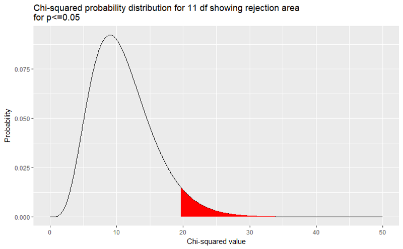
How did we change the rejection area in the graph? We used qchisq(0.05,11,lower.tail=FALSE instead of qchisq(0.025,11,lower.tail=FALSE. All the other code remained exactly the same.
Upcoming!
I will be writing separate posts on the Fisher and the Neyman-Pearson approaches to p-values. Both of these post-date Pearson. Again, I’ll use R to demonstrate the concepts so you can follow along.
As always, please feel free to amend the code as you wish.