
By Pier Paolo Ippolito
Probability Distributions play an important role in our daily lives. We commonly use them when trying to summarise and gain insights from different forms of data.
Because of this, they're quite an important topic in fields such as Mathematics, Computer Science, Statistics, and Data Science.
There are two main types of data: Numerical (for example integers and floats), and Categorical (for example strings of text).
Numerical data can also be in either of two forms:
- Discrete: this form of data can just take a limited number of values (like the number of clothes we have). We can infer probability mass functions from discrete data.
- Continuous: on the other hand, continuous data is used to describe more abstract concepts such as weight/distance which can take any fractional or real value. From continuous data we can instead infer probability density functions.
Probability mass functions can give us the probability that a variable is equal to a certain value. On the other hand, the values of probability density functions do not represent probabilities on their own, but instead first need to be integrated (within the considered range).
What is a Poisson Distribution?
Poisson Distributions are commonly used for two main purposes:
- Predicting how many times an event will take place within a chosen time period. This technique can be used for different risk analysis applications such as house insurance price estimation.
- Estimating a probability that an event might occur given how often it happened in the past (for example how likely it is that there will be a power-cut in the next two months).
Poisson Distributions let us be confident of the average time between the occurrence of different events. They can't, however, tell us the precise moment an event might take place (since processes usually have stochastic behaviour).
Linear vs non-linear systems
Natural systems can, in fact, be divided into two main categories: linear and non-linear (stochastic).
In linear systems, causes always precede their effect which creates a strong time precedence effect.
But this doesn't instead hold true when talking about non-linear systems, as small changes in the system's initial conditions can lead to unpredictable outcomes.
Considering how complex and chaotic our real world is, most processes are better described using non-linear systems, although linear approximations are sometimes possible.
Poisson Distributions can be modeled using the expression in the figure below, where λ is used to represent the expected number of events which can take place in the considered time-span.

The main characteristics which describe Poisson Processes are:
- Two events can't take place simultaneously.
- The average rate between event occurrence is overall constant.
- Events are independent of each other (if one happens, this does not have any influence on the probability that another event might take place).
- Events can take place any number of times (within the considered time-span).
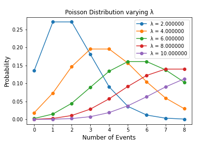
An example of a Poisson Distribution
In the figure below, you can see how varying the expected number of events (λ) which can take place in a period can change a Poisson Distribution. The image below has been simulated, making use of this Python code:
import numpy as np
import matplotlib.pyplot as plt
import scipy.stats as stats

# n = number of events, lambd = expected number of events
# which can take place in a period
for lambd in range(2, 12, 2):
    n = np.arange(0, 9)
    poisson = stats.poisson.pmf(n, lambd)
    plt.plot(n, poisson, '-o', label="λ = {:f}".format(lambd))
    plt.xlabel('Number of Events', fontsize=12)
    plt.ylabel('Probability', fontsize=12)
    plt.title("Poisson Distribution varying λ")
    plt.legend()
    plt.savefig('name.png')
Taking a closer look to this simulation, we can discover the following patterns:
- In each of the different cases, the number assigned to λ corresponds to the peak of the distribution, which then trails off moving further away from the peak.
- The more events that are expected to take place during the simulation, the greater the expected area under the distribution curve will be.
This type of simulation could, for example, be used to try to reduce the queuing time when going shopping to a supermarket.
The owner could create a record of how many customers visit the store at different times and on different days of the week in order to then fit this data to a Poisson Distribution.
In this way, it would be much easier to determine how many cashiers should be working at different times of the day/week in order to enhance the customer experience.
Wrapping up
In case you are interested in learning more about the applications of distributions in stochastic settings, more information is available here.
I hope you enjoyed this article, thank you for reading!
Contact me
If you want to keep updated with my latest articles and projects follow me on Medium and subscribe to my mailing list. These are some of my contacts details: