by Sachin Malhotra

Recursion Demystified

In order to understand recursion, you must first understand recursion.

Crazy, isn’t it ?

Well, I hope that by the end of this article you will feel much more confident about what recursion is and mainly, how we can come up with a recursive solution to a problem.

What is Recursion?

How do you explain recursion to a 4 year old? This is a pretty famous interview question, and there are loads of answers available on the web. We won’t answer this question as it is too mainstream.

If you are as clever as I am ??, you would explain recursion to someone one year younger than you. Have them explain recursion to someone one year younger than them. Continue until you have a 5 year old explaining recursion to a 4 year old. Done. [Source: reddit].

In programming terms, recursion is

A function calling itself.

The above function does no useful work as such, but it does demonstrate recursion. The recursive relation above would be

T(N) = T(N - 1) + O(1)

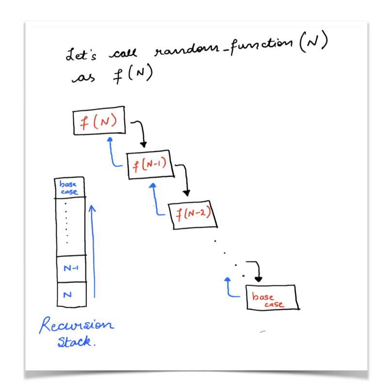
This simply means that the execution for the call to random_function(n) cannot proceed until the call to random_function(n-1) is completed and so on.

Essentially, we delay the execution of the current state of the function until another call to the same function has completed and returned it’s result.

The compiler keeps on saving the state of the function call now and then moves onto the next function call and so on. So, the compiler saves function states onto a stack and uses that for computations and backtracking.

Essentially, if a problem can be broken down into similar subproblems which can be solved individually, and whose solutions can be combined together to get the overall solution, then we say that there might exist a recursive solution to the problem.

Instead of clinging to this seemingly old definition of recursion, we will look at a whole bunch of applications of recursion. Then hopefully things will be clear.

Factorial of a Number

Let us see how we can find out the factorial of a number. Before that, let’s see what the factorial of a number represents and how it is calculated.

factorial(N) = 1 * 2 * 3 * .... * N - 1 * N

Simply put, the factorial of a number is just the product of terms from 1 to the number N multiplied by one another.

We can simply have a for loop from 1 to N and multiply all the terms iteratively and we will have the factorial of the given number.

But, if you look closely, there exists an inherent recursive structure to the factorial of a number.

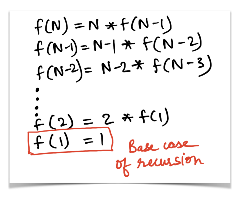
factorial(N) = N * factorial(N - 1)

It’s like offloading the computation to another function call operating on a smaller version of the original problem. Let’s see how this relation would unfold to verify if the solution here matches the one provided by the for loop.

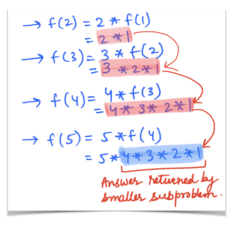
So, it is clear from the two figures above that the recursive function that we defined earlier,

factorial(N) = N * factorial(N - 1)

is indeed correct. Have a look at the Python code snippet used to find the factorial of a function, recursively.

This example was pretty simple. Let us consider a slightly bigger but standard example to demonstrate the concept of recursion.

Fibonacci Sequence

You must be already familiar with the famous fibonacci sequence. For those of you who have’t heard about this sequence or seen an example before, lets have a look.

1 1  2   3     5           8                       13 ..... 

Let us look at the formula for calculating the n^th fibonacci number.

F(n) = F(n - 1) + F(n - 2)where F(1) = F(2) = 1

Clearly, this definition of the fibonacci sequence is recursive in nature, since the n^th fibonacci number is dependent upon the previous two fibonacci numbers. This means dividing the problem into smaller subproblems, and hence recursion. Have a look at the code for this:

Every recursive problem must have two necessary things:

1. The recurrence relation defining the states of the problem and how the main problem can be broken down into smaller subproblems. This also includes the base case for stopping the recursion.
2. A recursion tree that showcases the first few, if not all calls to the function under consideration. Have a look at the recursion tree for the fibonacci sequences’ recursive relation.

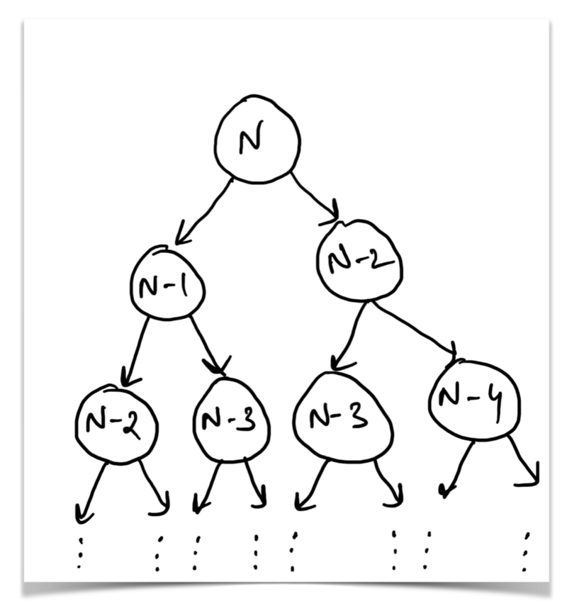
The recursion tree shows us that the results obtained from processing the two subtrees of the root N can be used to compute the result for the tree rooted at N. Similarly for other nodes.

The leaves of this recursion tree would be fibonacci(1) or fibonacci(2) both of which represent the base cases for this recursion.

Now that we have a very basic grasp of recursion, what a recurrence relation is, and the recursion tree, let’s move onto something more interesting.

Examples!

I strongly believe in solving umpteen number of examples for any given topic in programming to become a master of that topic. The two examples we considered (Factorial of a number and the Fibonacci sequence) had well defined recurrence relations. Let us look at a few examples where the recurrence relation might not be so obvious.

Height of a Tree

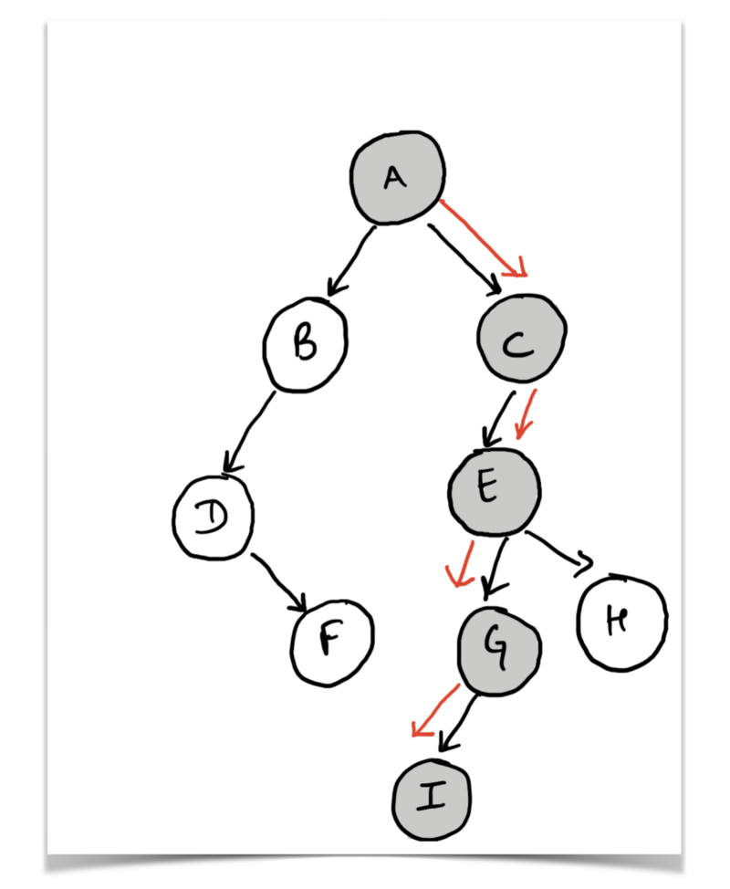
To keep things simple for this example, we will only consider a binary tree. So, a binary tree is a tree data structure in which each node has at most two children. One node of the tree is designated as the root of the tree, for example:

Let’s define what we mean by the height of the binary tree.

Height of the tree would be the length of the longest root to leaf path in the tree.

So, for the example diagram displayed above, considering that the node labelled as A as the root of the tree, the longest root to leaf path is A → C → E → G → I . Essentially, the height of this tree is 5 if we count the number of nodes and 4 if we just count the number of edges on the longest path.

Now, forget about the entire tree and just focus on the portions highlighted in the diagram below.

The above figure shows us that we can represent a tree in the form of its subtrees. Essentially, the structure to the left of node A and the structure to the right of A is also a binary tree in itself, just smaller and with different root nodes. But, they are binary trees nonetheless.

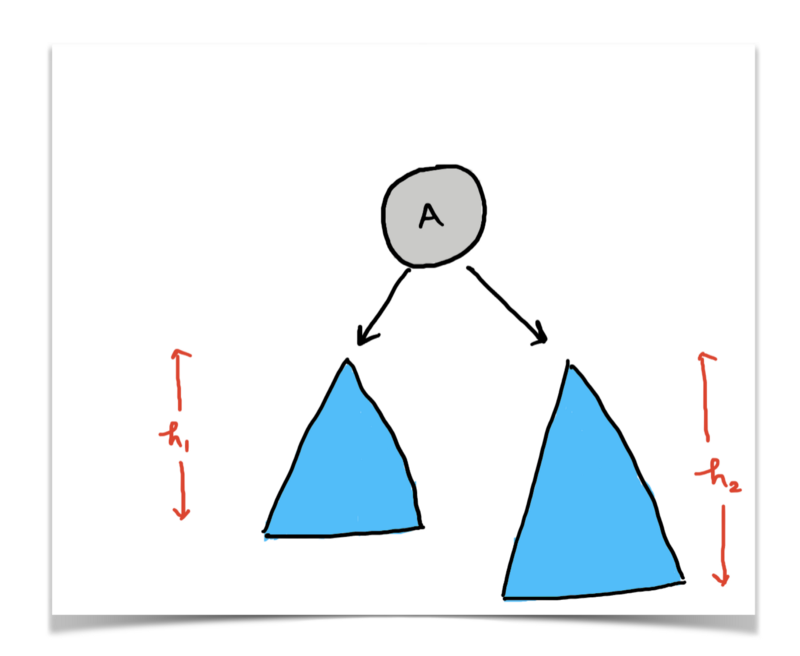
What information can we get from these two subtrees that would help us find the height of the main tree rooted at A ?

If we knew the height of the left subtree, say h1, and the height of the right subtree, say h2, then we can simply say that the maximum of the two + 1 for the node A would give us the height of our tree. Isn’t that right?

Formalizing this recursive relation,

height(root) = max(height(root.left), height(root.right)) + 1

So, that’s the recursive definition of the height of a binary tree. The focus is on binary here, because we used just two children of the node root represented by root.left and root.right. But, it is easy to extend this recursive relation to an n-ary tree. Let’s take a look at this in code.

The problem here was greatly simplified because we let recursion do all the heavy lifting for us. We simply used optimal answers for our subproblems to find a solution to our original problem.

Let’s look at another example that can be solved on similar lines.

Number of Nodes in a Tree

Here again, we will consider a binary tree for simplicity, but the algorithm and the approach can be extended to any kind of tree essentially.

The problem is itself very self explanatory. Given the root of a binary tree, we need to determine the total number of nodes in the tree. This question and the approach we will come up with here are very similar to the previous one. We just have to make minuscule changes and we will have the number of nodes in the binary tree.

Take a look at the diagram below.

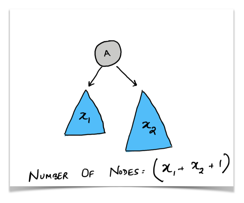
The diagram says it all. We already know that a tree can be broken down into smaller subtrees. Here again, we can ask ourselves,

What information can we get from these two subtrees that would help us find the number of nodes in the tree rooted at A?

Well, if we knew the number of nodes in the left subtree and the number of nodes in the right subtree, we can simply add them up and add one for the root node and that would give us the total number of nodes.

Formalizing this we get,

number_of_nodes(root) = number_of_nodes(root.left) +        number_of_nodes(right) + 1

If you look at this recursion and the previous one, you will find that they are extremely similar. The only thing that is varying is what we do with the information we obtained from our subproblems and how we combined them to get some answer.

Now that we have seen a couple of easy examples with a binary tree, let’s move onto something less trivial.

Merge Sort

Given an array of numbers like

4 2 8 9 1 5 2

we need to come up with a sorting technique that sorts them either in ascending or descending order. There are a lot of famous sorting techniques out there for this like Quick Sort, Heap Sort, Radix Sort and so on. But we are specifically going to look at a technique called the Merge Sort.

It’s possible that a lot of you are familiar with the Divide and Conquer paradigm, and this might feel redundant. But bear with me and read on!

The idea here is to break it down into subproblems.

That’s what the article is about right ? ?

What if we had two sorted halves of the original array. Can we use them somehow to sort the entire array?

That’s the main idea here. The task of sorting an array can be broken down into two smaller subtasks:

• sorting two different halves of the array
• then using those sorted halves to obtain the original sorted array

Now, the beauty about recursion is, you don’t need to worry about how we will get two sorted halves and what logic will go into that. Since this is recursion, the same method call to merge_sort would sort the two halves for us. All we need to do is focus on what we need to do once we have the sorted haves with us.

Let’s go through the code:

At this point, we trusted and relied on our good friend recursion and assumed that left_sorted_half and right_sorted_half would in fact contain the two sorted halves of the original array.

So, what next?

The question is how to combine them somehow to give the entire array.

The problem now simply boils down to merging two sorted arrays into one. This is a pretty standard problem and can be solved by what is known as the “two finger approach”.

Take a look at the pseudo code for better understanding.

let L and R be our two sorted halves. let ans be the combined, sorted array

l = 0 // The pointer for the left halfr = 0 // The pointer for the right halfa = 0 // The pointer for the array ans

while l < L.length and r < R.length {      if L[l] < R[r] {           ans[a] = L[l]           l++       } else {           ans[a] = R[r]           r++      }}

copy remaining array portion of L or R, whichever was longer, into ans.

Here we have two pointers (fingers), and we position them at the start of the individual halves. We check which one is smaller (that is, which value pointed at by the finger is smaller), and we add that value to our sorted combined array. We then advance the respective pointer (finger) forward. In the end we copy the remaining portion of the longer array and add it to the back of the ans array.

So, the combined code for merge-sort is as follows:

We will do one final question using recursion and trust me, it’s a tough one and a pretty confusing one. But before moving onto that, I will iterate the steps I follow whenever I have to think of a recursive solution to a problem.

Steps to come up with a Recursive Solution

1. Try and break down the problem into subproblems.

2. Once you have the subproblems figured out, think about what information from the call to the subproblems can you use to solve the task at hand. For example, the factorial of N — 1 to find the factorial of N , height of the left and right subtrees to find the height of the main tree, and so on.

3. Keep calm and trust recursion! Assume that your recursive calls to the subproblems will return the information you need in the most optimal fashion.

4. The final step in this process is actually using information we just got from the subproblems to find the solution to the main problem. Once you have that, you’re ready to code up your recursive solution.

Now that we have all the steps lined up, let’s move on to our final problem in this article. It’s called Sum of Distances in a Tree.

Sum of Distances in a Tree

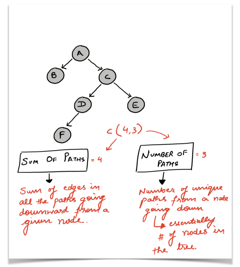
Let’s look at what the question is asking us to do here. Consider the following tree.

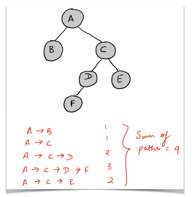
In the example above, the sum of paths for the node A (the number of nodes on each path from A to every other vertex in the tree) is 9. The individual paths are mentioned in the diagram itself with their respective lengths.

Similarly, consider the sum of distances for the node C.

C --> A --> B (Length 2)C --> A (Length 1)C --> D (Length 1)C --> E (Length 1)C --> D --> F (Length 2)Sum of distances (C) = 2 + 1 + 1 + 1 + 2 = 7

This is known as the sum of distances as defined for just a single node A or C. We need to calculate these distances for each of the nodes in the tree.

Before actually solving this generic problem, let us consider a simplified version of the same problem. It says that we just need to calculate the sum of distances for a given node, but we will only consider the tree rooted at the given node for calculations.

So, for the node C, this simplified version of the problem would ask us to calculate:

C --> D (Length 1)C --> E (Length 1)C --> D --> F (Length 2)Simplified Sum of Distances (C) = 1 + 1 + 2 = 4

This is a much simpler problem to tackle recursively and would prove to be useful in solving the original problem.

Consider the following simple tree.

The nodes B and C are the children of the root (that is, A).

We are trying to see what information can we use from subproblems (the children) to compute the answer for the root A .

Note: here we simply want to calculate the sum of paths for a given node X to all its successors in its own subtree (the tree rooted at the node X).

There are no downwards going paths from the node B, and so the sum of paths is 0 for the node B in this tree. Let’s look at the node C . So this node has 3 different successors in F, D and E . The sum of distances are as follows:

C --> D (Path containing just 1 edge, hence sum of distances = 1)C --> D --> F (Path containing 2 edges, hence sum of distances = 2)C --> E (Path containing just 1 edge, hence sum of distances = 1)

The sum of all the paths from the node C to all of its decedents is 4, and number of such paths going down is 3.

Note the difference here. The sum_of_distances here counts the number of edges in each path — with each edge repeating multiple times, probably because of their occurrence on different paths — unlike number_of_paths , which counts, well, the number of paths ?.

If you look closely, you will realize that the number of paths going down is always going to be the number of nodes in the tree we are considering (except the root). So, for the tree rooted at C, we have 3 paths, one for the node D, one for E, and one for F. This means that the number of paths from a given node to the successor nodes is simply the total number of descendent nodes since this is a tree. So, no cycles or multiple edges.

Now, consider the node A. Let us look at all the new paths that are being introduced because of this node A. Forget the node B for now and just focus on the child node C corresponding to A. The new sets of paths that we have are:

A --> C (Path containing just 1 edge, hence sum of distances = 1)A --> (C --> D)    (Path containing 2 edges, hence sum of distances = 2)A --> (C --> E)    (Path containing 2 edges, hence sum of distances = 2)A --> (C --> D --> F) (Path containing 3 edges, hence sum of distances = 3)

Except for the first path A → C, all the others are the same as the ones for the node C, except that we have simply changed all of them and incorporated one extra node A.

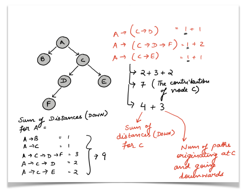
If you look at the diagram above you will see a tuple of values next to each of the nodes A, B, and C.

(X, Y) where X is the number of paths originating at that node and going down to the decedents. Y is the sum of distances for the tree rooted at the given node. 

Since the node B doesn’t have any further children, the only path it is contributing to is the path A -->; B to A's tuple of (5, 9) above. So let’s talk about C.

C had three paths going to its successors. Those three paths (extended by one more node for A) also become three paths from A to its successors, among others.

N-Paths[A] = (N-Paths[C] + 1) + (N-Paths[B] + 1)

That is the exact relation we are looking for as far as the number of paths (= number of successor nodes in the tree) are concerned. The 1 is because of the new path from the root to it’s child, that is A -->; C in our case.

N-Paths[A] = 3 + 1 + 0 + 1 = 5

As far as the sum of distances is concerned, take a look at the diagram and the equations we just wrote. The following formula becomes very clear:

Sum-Dist[A] = (N-Paths[C] + 1 + Sum-Dist[C]) + (N-Paths[B] + 1 + Sum-Dist[B])

Sum-Dist[A] = (3 + 1 + 4 + 0 + 1 + 0) = 9

The main thing here is N-Paths[C] + Sum-Dist[C] . We sum these up because all of the paths from C to its descendants ultimately become the paths from A to its descendants — except that they originate at A and go through C, and so each of the path lengths are increased by 1. There are N-Paths[C] paths in all originating from C and their total length is given by Sum-Dist[C] .

Hence the tuple corresponding to A = (5, 9). The Python code for the algorithm we discussed above is as follows:

The Curious Case of the Visited Dictionary :/

If you look at the code above closely, you’ll see this:

# Prevents the recursion from going into a cycle.        self.visited[vertex] = 1

The comment says that this visited dictionary is for preventing the recursion from entering a cycle.

If you’ve paid attention til now, you know that we are dealing with a tree here.

The definition of a tree data structure doesn’t allow cycles to exist. If a cycle exists in the structure, then it is no longer a tree, it becomes a graph. In a tree, there is exactly one path between any two pair of vertices. A cycle would mean there is more than one path between a pair of vertices. Look at the figures below.

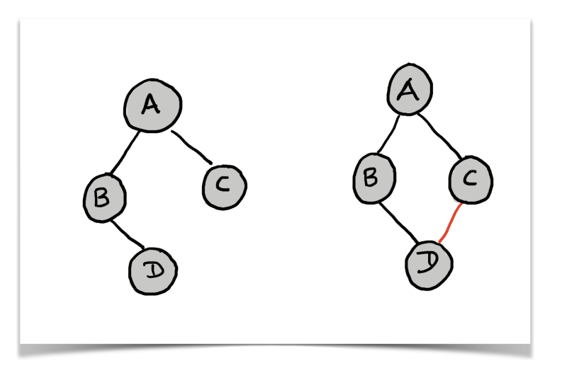
The structure on the left is a tree. It has no cycles in it. There is a unique path between any two vertices.

The structure on the right is a graph, there exists a cycle in the graph and hence there are multiple paths between any pair of vertices. For this graph, it so happens that any pair of vertices have more than one path. This is not necessary for every graph.

Almost always, we are given the root node of the tree. We can use the root node to traverse the entire tree without having to worry about any cycles as such.

However, if you’ve read the problem statement clearly, it does not state anything about root of the tree.

That means that there is no designated root for the tree given in the question. This could mean that a given tree can be visualized and processed in so many different ways depending upon what we consider as the root. Have a look at multiple structures for the same tree but with different root nodes.

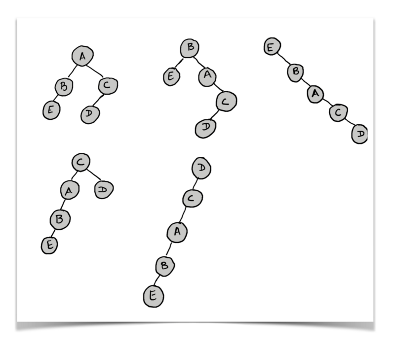
So many different interpretations and parent child relationships are possible for a given unrooted tree.

So, we start with the node 0 and do a DFS traversal of the given structure. In the process we fix the parent child relationships. Given the edges in the problem, we construct an undirected graph-like structure which we convert to the tree structure. Taking a look at the code should clear up some of your doubts:

Every node would have one parent. The root won’t have any parent, and the way this logic is, the node 0 would become the root of our tree. Note that we are not doing this process separately and then calculating the sum of distances downwards. Given a tree, we were trying to find, for every node, the simplified sum of distances for the tree rooted at that node.

So, the conversion from the graph to the tree happens in one single iteration along with finding out the sum of distances downwards for each and every node.

I posted the code again so that the visited dictionary makes much more sense now. So, one single recursion doing all that for us. Nice!

Bringing it all together

Now that we have our tree structure defined, and also the values of sum of distances going downward defined for us, we can use all of this information to solve the original problem of Sum of Distances in a Tree.

How do we do that? It’s best to explain this algorithm with the help of an example. So we will consider the tree below and we will dry run the algorithm for a single node. Let’s have a look at the tree we will be considering.

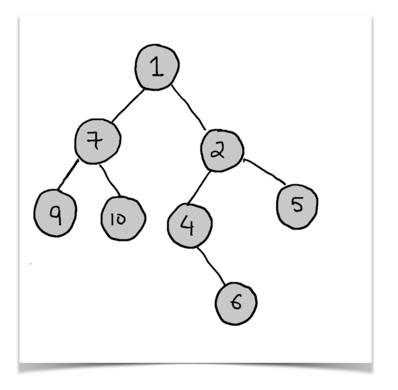
The node for which we want to find the sum of distances is 4. Now, if you remember the simpler problem we were trying to solve earlier, you know that we already have two values associated with each of the nodes:

1. distances_down Which is the sum of distances for this node while only considering the tree beneath.
2. number_of_paths_down which is the number of paths / nodes in the tree rooted at the node under consideration.

Let’s look at the annotated version of the above tree. The tree is annotated with tuples (distances_down, number_of_paths_down) .

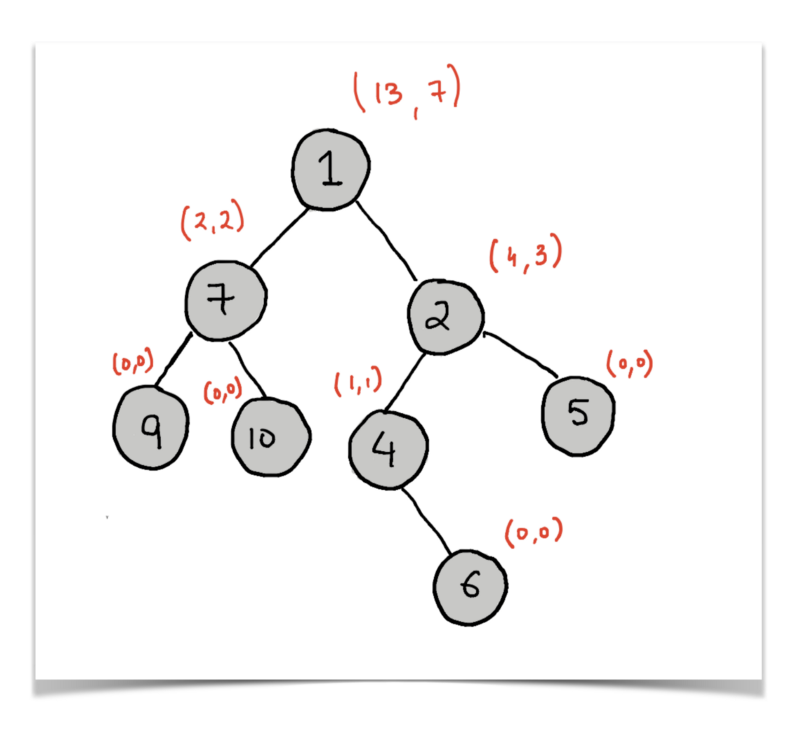
Let’s call the value we want to compute for each node as sod which means sum of distances, which is what the question originally asks us to compute.

Let us assume that we have already computed the answer for the parent node of 4 in the diagram above. So, we now have the following information for the node labelled 2 (the parent node) available:

(sod, distances_down, number_of_paths_down) = (13, 4, 3)

Let’s rotate the given tree and visualize it in a way where 2 is the root of the tree essentially.

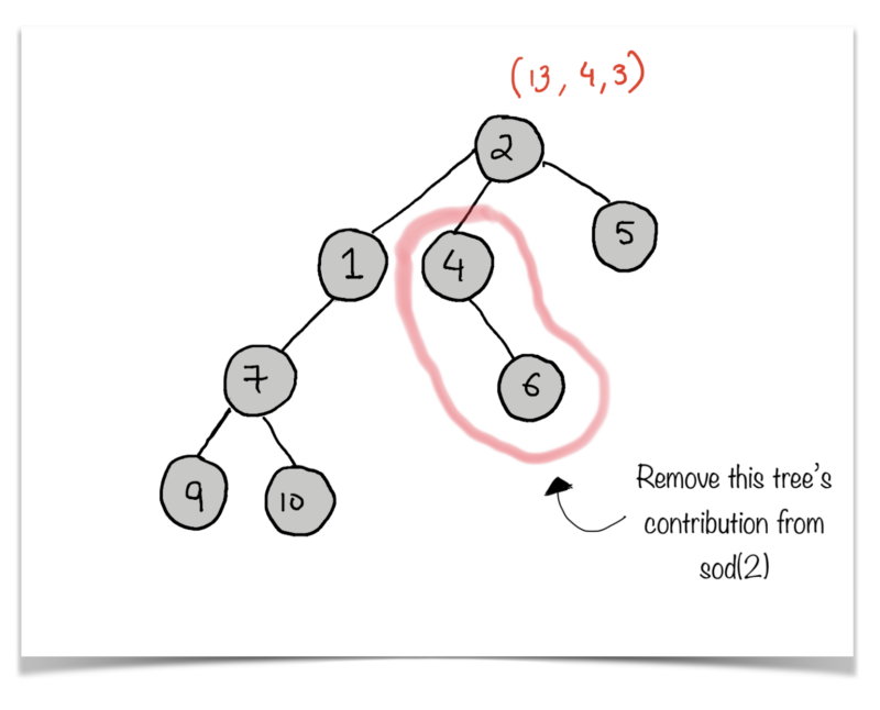
Now, we want to remove the contribution of the tree rooted at 4 from sod(2). Let us consider all of the paths from the parent node 2 to all other nodes except the ones in the tree rooted at 4 .

2 --> 5 (1 edge)2 --> 1 (1 edge)2 --> 1 -->7 (2 edges)2 --> 1 --> 7 --> 9 (3 edges)2 --> 1 --> 7 --> 10 (3 edges)

Number of nodes considered = 6Sum of paths remaining i.e. sod(2) rem = 1 + 1 + 2 + 3 + 3 = 10

Let’s see how we can use the values we already have calculated to get these updated values.

* N = 8 (Total number of nodes in the tree. This will remain the same for every node. )* sod(2) = 13

* distances_down[4] = 1* number_of_paths_down[4] = 1

* (distances_down[4] does not include the node 4 itself)N - 1 - distances_down[4] = 8 - 1 - 1 = 6

* sod(2) - 1 - distances_down[4] - number_of_paths_down[4] = 13 - 1 - 1 - 1 = 10

If you remember this from the function we defined earlier, you will notice that the contribution of a child node to the two values distances_down and number_of_paths_down is n_paths + 1 and n_paths + s_paths + 1 respectively. Naturally, that is what we subtract to obtain the remaining tree.

sod(4) represents the sum of edges on all the paths originating at the node 4 in the tree above. Let’s see how we can find this out using the information we have calculated till now.

distances_down[4] represents the answer for the tree rooted at the node 4 but it only considers paths going to its successors, that is all the nodes in the tree rooted at 4. For our example, the successor of 4 is the node 6. So, that will directly add to the final answer. Let’s call this value own_answer . Now, let’s account for all the other paths.

4 --> 2 (1 edge)4 --> 2 --> 5 (1 + 1 edge)4 --> 2 --> 1 (1 + 1 edge)4 --> 2 --> 1 -->7 (1 + 2 edges)4 --> 2 --> 1 --> 7 --> 9 (1 + 3 edges)4 --> 2 --> 1 --> 7 --> 10 (1 + 3 edges)own_answer = 1

sod(4) = 1 + 1 + 2 + 2 + 3 + 4 + 4 = 17

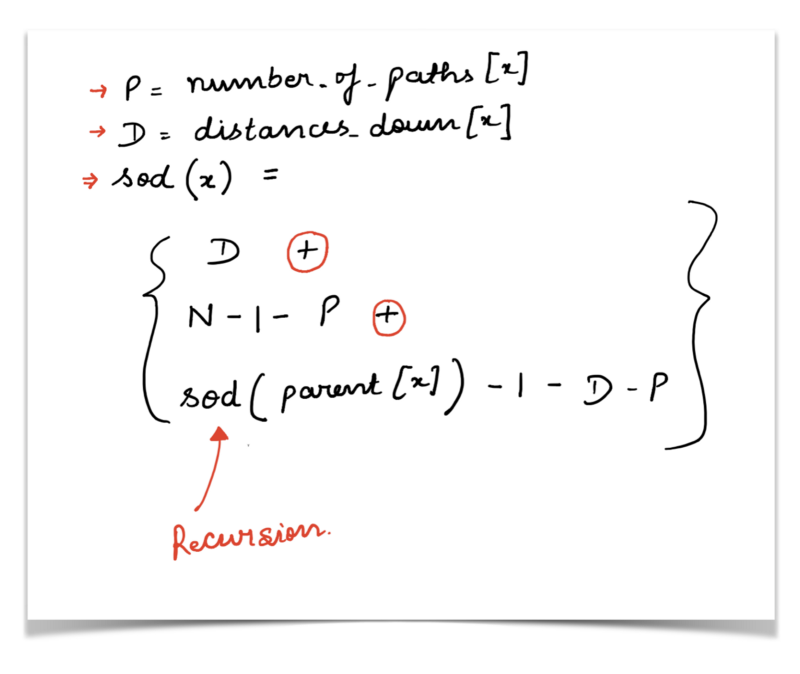
sod(4) = own_answer + (N - 1 - distances_down[4]) + (sod(2) - 1 - distances_down[4] - number_of_paths_down[4]) = 1 + 6 + 10 = 17

Before you go bonkers and start doing this, let’s look at the code and bring together all of the things we discussed in the example above.

The recursive relation for this portion is as follows:

Did I just see “MEMOIZATION” in the code?

Yes, indeed you did!

Consider the following example tree:

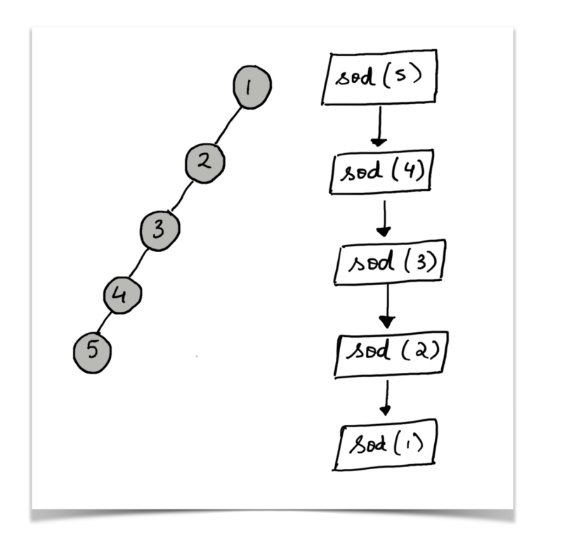
The question asks us to find the sum of distances for all the nodes in the given tree. So, we would do something like this:

for i in range(N):    ans.append(find_distances(N))

But, if you look at the tree above, the recursive call for the node 5 would end up calculating the answers for all the nodes in the tree. So, we don’t need to recalculate the answers for the other nodes again and again.

Hence, we end up storing the already calculated values in a dictionary and use that in further calculations.

Essentially, the recursion is based on the parent of a node, and multiple nodes can have the same parent. So, the answer for the parent should only be calculated once and then be used again and again.

If you’ve managed to read the article this far (not necessarily in one stretch ?), you’re awesome ?.

If you found this article helpful, share as much as possible and spread the ?. Cheers!