
![The Math Behind Artificial Intelligence: A Guide to AI Foundations [Full Book]](https://cdn.hashnode.com/res/hashnode/image/upload/v1767723634484/4748bd8a-26a1-4d9c-89c3-1a6d07bde69e.png)
"To understand is to perceive patterns." - Isaiah Berlin
This is not a math book filled with complex formulas, theorems, and concepts that are hard to grasp.
Instead, it’s a detailed guide where we’ll break complex ideas down into simpler terms.
Even if you only have a general understanding of algebra, you should be able to easily follow along.
Here’s what we’ll cover:
Chapter 5: Multivariable Calculus - Change in Many Directions
Chapter 6: Probability & Statistics - Learning from Uncertainty
Chapter 7: Optimization Theory - Teaching Machines to Improve
Chapter 1: Background on this Book
The Objective Here
My objective in this book is simple: Explain the key mathematical ideas you need to grasp in order to deeply understand AI and train machine learning models.
So you might be wondering: Why is it important to have a good math foundation before creating these models?
Well, there are many reasons, but some are:
It gives you the capacity to understand new AI research on your own.
You can use this same foundation to study other STEM concepts like signal theory and advanced statistical methods.
It helps you understand that AI models are just a mixture of different math ideas working together and gives you insight into how new innovations make LLMs more efficient.
It gives you a foundation so you know how to calibrate AI models and even create derivative models.
These skills are also important for startup founders, especially in Silicon Valley. Many startups begin with APIs or API wrappers but eventually need their own AI solutions.
Outsourcing all AI isn't ideal. This book will help you understand AI foundations so you can design better growth strategies and communicate effectively with investors – especially those who were successful technical co-founders.
Why is This Book About AI Different?
In this book, we’ll look at AI from an engineering perspective. This differs from the typical computer science approach to AI that most introductory courses take.
In doing so, I won’t spend a lot of time explaining formulas and theorems. Instead, I’ll explain their importance, how and why they are applied the way they are.
In this way, I hope to offer a unique viewpoint that emphasizes the engineering principles and good practices that underlie all modern AI technologies.
I will also explain how many of these strange math ideas make billion dollar industries possible.
We’ll start with the fundamentals: the structure of the areas of mathematics and AI. After that, we’ll look at the four subareas of math that make AI possible:
Linear Algebra
Calculus
Probability Theory and Statistics
Optimization Theory
After going through all the math, we’ll connect it with the foundation of ChatGPT and all of these large language models.
This way, you’ll get a basic foundation in key math concepts that, when mixed together like the ingredients of a cake, make all AI models possible.
By knowing where the ideas come from, you’ll develop a system-level understanding of AI and a first-principles approach.
So just keep in mind that, even though concepts like integral calculus and eigenvalues/eigenvectors might not be widely used in AI, they’ll help you develop these system-level and first-principle approaches.
Also, this book will be a work in progress. After its first release, I’ll seek feedback on things I need to perfect, chapters to add, and so on.
Here is my email for any feedback you might have: monteiro.t@northeastern.edu
And here is the book’s GitHub repository with all code: https://github.com/tiagomonteiro0715/The-Math-Behind-Artificial-Intelligence-A-Guide-to-AI-Foundations
Let Me Introduce Myself
My name is Tiago Monteiro, an electrical and computer engineer and AI master's degree student at Northeastern University's Silicon Valley campus. I have authored 20+ articles with 240K+ views here on freeCodeCamp on math, AI, and tech.
If you’d like to know more about my background, I’ll share that at the end of the book.
Prerequisites
In terms of minimum requirements, you only need to know the basics of mathematics and programming:
Basic algebra and what functions and the coordinate system are.
You should be able to read Python code and understand things like variables, functions, and loops.
Chapter 2: The Architecture of Mathematics

Math is more than numbers. It’s the science of locating complex patterns that shape our world. To truly understand math, we must look beyond numbers and formulas to grasp its structures.
This chapter aims to show math as a growing tree of ideas, a living system of logic, not just formulas to memorize. With analogies, history, and code examples, I want to help you understand math deeply and how to apply it to programming.
I’ve included code examples to connect theory and practice, showing how math ideas apply to real problems. Whether you're new to advanced math or are more experienced, these examples will help you apply math in programming.
This way, before we start going over the different math pillars that sustain AI, you will understand the structure of the field.
The Tree of Mathematics: How Everything Connects

Photo by Lerkrat Tangsri
Imagine math as a vast, ever-growing tree.
The roots are the foundations: logic and set theory. From these roots, the main fields emerge: arithmetic, algebra, geometry, and analysis.
As the tree branches out, new subfields like topology and abstract algebra appear. Sometimes branches connect with each other.
This tree keeps growing in many directions. History shows that sometimes it grows rapidly due to scientific discoveries, while at other times, growth is slow.
And you might wonder: How many more branches and connections between them will keep appearing?
A Quick History of Mathematics: From Counting to Infinity
The first mathematical ideas emerged independently in ancient civilizations, such as:
India's invention of zero
Islamic algebraic advances
Greek geometric rigor
Great mathematicians developed and shared these ideas through writing and lectures. Over time, new generations built on these ideas, creating new branches of mathematics. This endless growth is why Isaac Newton wrote to Robert Hooke in 1675:
“If I have seen further, it is by standing on the shoulders of giants.”
He meant that by working from previous knowledge, he was able to create and (re)discover new ideas.
Yet, the real power of math lies in practicing it over and over and studying it more and more deeply.
As one of my professors once pointed out:
“More important than knowing the theorems is knowing the ideas behind them and the history of how they were created.”
To solve problems, it's often necessary to think from first principles, and math teaches this. Math is not just an academic topic. It’s a global language for scientists and engineers.
By preserving and sharing it, new math can grow from old ideas, allowing the tree to keep expanding.
Foundations of Relativity: How Einstein Used Math to Understand Space and Time

Photo by Pixabay
Albert Einstein developed the general and special theories of relativity, which impact:
GPS and global communication
Satellite telecommunications
Space exploration and satellite launches
And more.
But this was only possible by combining geometry with calculus, known as differential geometry. This field evolved over centuries, thanks to many great mathematicians. Here are a few of them, though the list is not exhaustive:
Euclid (circa 300 BCE): Contributed to geometry, laying the groundwork for later mathematical systems
Archimedes (circa 287–212 BCE): Pioneered the understanding of volume, surface area, and the principles of mechanics
René Descartes (1596–1650): Developed Cartesian coordinates and analytical geometry
Isaac Newton (1642–1727) & Gottfried Wilhelm Leibniz (1646–1716): Newton’s laws of motion and gravitation, alongside Leibniz’s development of calculus, formed the basis of classical mechanics that Einstein sought to extend and modify in his theory of relativity.
Leonhard Euler (1707–1783): Contributed to the development of differential equations, which are essential in the mathematical foundations of physics.
Gaspard Monge (1746–1818): The father of differential geometry and pioneer in descriptive geometry
Carl Friedrich Gauss (1777–1855): Made groundbreaking advances in geometry, including the concept of curved surfaces.
Bernhard Riemann (1826–1866): Introduced Riemannian geometry, a branch of differential geometry.
Going back to Albert Einstein, he saw what no one else in his time saw, thanks to these great math giants and countless others.
Gödel’s Biggest Paradox: Can Math Explain Itself?
The biggest paradox in math, discovered by Kurt Gödel, is his incompleteness theorems. They show that in any consistent formal system capable of simple arithmetic, there are true statements that cannot be proven within the system.
This means there are limits to what can be proven as true or false. For mathematicians, this implies that some truths are beyond formal proofs, yet we assume they are true. It demonstrates that no matter how much effort or AI is used, some things remain unprovable, known only through approximations and non-exact methods.
What About Applied Math and Engineering?
Applied math and engineering involve adapting the pure math ideas in real-world scenarios.
Actually, in many cases, it’s the combination of many math ideas.
Let’s consider some examples:
In harmonic analysis, Laplace, Fourier, and Z-transforms are a way to see the same thing in a new domain to get new insights. In this case, integrals are used to make this mapping possible.
Principal component analysis (PCA) is a widely used tool in data science. Yet, it is a mixture of linear algebra (in PCA, eigenvalues) with optimization (order eigenvalues that represent more data with less data) in order to make datasets shorter.
In machine learning, logistic regression is a mixture of calculus with statistics and probability.
In deep learning, neural networks are just many matrices multiplying and updating themselves that adapt to model a dataset representing a system. This optimization of matrix values happens with activation functions, a gradient descent-based optimization method (tells how much values need to change), and backpropagation (applies those alterations to all matrix values).
But the best example of this fusion of math in engineering is in control theory. Control theory is the study of the architecture of systems. From trains to cars to airplanes, everything is based on control theory. It’s everywhere, in nearly all modern electronic devices. In electric circuits, control theory is also used heavily to guarantee circuit stability in the face of electric disturbances.
So as you can probably start to see, many of the tools we now have are just a mixture of many pure math ideas – like different recipes. In essence, applied math is the application of pure math as “ingredients“ in "recipes" to solve problems.
So, we’ve explored the structure and evolution of mathematics. But it’s important to see how we can apply these ideas in real life. Pure math makes the framework, and applied math applies that framework to solve problems. To understand this, we’ll examine two code examples that show how you can use math ideas as programming tools.
Code Examples: Analytical and Numerical Approaches
These code examples demonstrate a couple ways you can use Python to solve math equations.
In the first code example, we’ll solve the problem in the same way that kids in school solve math exercises: essentially, by hand with a pencil. In the second example, we’ll solve the problem using numerical analysis.
Example 1: Solve a Problem Analytically
In this problem, we need to find the values of the variables x and y. So we’ll be moving variables from left to right to find their values.
When we solve math problems analytically, like we did in school, we are manipulating symbols to get exact values. Often these symbols are x, y, and z.
The code below solves a system of two equations with two unknowns variables, x and y.
We will use the SymPy Python library to do this. It’s mainly used for symbolic mathematics.
from sympy import symbols, Eq, solve

x, y = symbols('x y')
eq1 = Eq(2*x + 3*y, 6)
eq2 = Eq(-x + y, 1)

solution = solve((eq1, eq2), (x, y))
print(solution)

Once again with this code we are finding the values of the variables x and y.
Essentially, we’re finding x and y based on this equation:
$$\begin{align} 2x + 3y &= 6 \ -x + y &= 1 \end{align}$$
Which gives us the following result:
{x: 3/5, y: 8/5}
Or:
x= 0.6
y = 1.6
When we say that we’re solving this analytically, it means that we’re finding an exact mathematical solution using formulas or equations.
But many times, problems are harder and can be solved by adding symbols to the right or left of the equation. Sometimes, there can be so many symbols and transformed versions of them, with things like derivatives and integrals, that it can become very hard to manage and takes a lot of time.
For example, let’s look at this partial differential equation:
$$\begin{cases} \frac{\partial u}{\partial t} = \alpha \frac{\partial^2 u}{\partial x^2}, & 0 < x < L, , t > 0 \ u(0,t) = 0, & t > 0 \ u(L,t) = 0, & t > 0 \ u(x,0) = f(x), & 0 < x < L \end{cases}$$
It can be solved with an analytical method call separation of variables.
But it requires many steps, and it’s easy to make mistakes. Even engineers who learned this often struggle to remember the process later.
When I first encountered this type of math exercise in my electrical and computer engineering degree back in Portugal, it took me 20 to 30 minutes to solve it.
For this reason, there's a branch of mathematics called numerical analysis that focuses on finding approximations of existing formulas. It helps solve problems faster. This is the method we'll explore next.
Example 2: Solve Numerically (Approximation)
Now let’s solve a different problem: we’re going to find the values of each of the 5 variables:
$$\begin{bmatrix} 3 & 2 & -1 & 4 & 5 \ 1 & 1 & 3 & 2 & -2 \ 4 & -1 & 2 & 1 & 0 \ 5 & 3 & -2 & 1 & 1 \ 2 & -3 & 1 & 3 & 4 \end{bmatrix} \times \begin{bmatrix} x_1 \ x_2 \ x_3 \ x_4 \ x_5 \end{bmatrix} = \begin{bmatrix} 12 \ 5 \ 7 \ 9 \ 10 \end{bmatrix}$$
Solving this by hand will take some time…but with Python code, it’s very fast.
We’ll also use the SciPy Python library for this example.
Let’s solve the system numerically:
import numpy as np
from scipy.linalg import solve

A = np.array([[3, 2, -1, 4, 5],
              [1, 1, 3, 2, -2],
              [4, -1, 2, 1, 0],
              [5, 3, -2, 1, 1],
              [2, -3, 1, 3, 4]])

b = np.array([12, 5, 7, 9, 10])

solution = solve(A, b)

print(solution)

Which corresponds to this operation:
$$\begin{bmatrix} 3 & 2 & -1 & 4 & 5 \ 1 & 1 & 3 & 2 & -2 \ 4 & -1 & 2 & 1 & 0 \ 5 & 3 & -2 & 1 & 1 \ 2 & -3 & 1 & 3 & 4 \end{bmatrix} \times \begin{bmatrix} x_1 \ x_2 \ x_3 \ x_4 \ x_5 \end{bmatrix} = \begin{bmatrix} 12 \ 5 \ 7 \ 9 \ 10 \end{bmatrix}$$
Again, it takes time to solve this and it’s very easy to make a simple mistake.
But in this code example, this line of code:
solution = solve(A, b)
Uses the solve method from SciPy:
from scipy.linalg import solve
It’s a method that helps you find the values of x in an equation A⋅x=b, where A is a square grid of numbers and b is a list of numbers. That gives us the following:
[ 1.35022026 -0.79955947 -1.17180617 3.14317181 -0.83920705]
Which corresponds to:
$$\begin{bmatrix} x_1 \ x_2 \ x_3 \ x_4 \ x_5 \end{bmatrix} = \begin{bmatrix} 1.35022026 \ -0.79955947 \ -1.17180617 \ 3.14317181 \ -0.83920705 \end{bmatrix}$$
And is the same thing as:
$$\begin{align} x_1 &= 1.35022026 \ x_2 &= -0.79955947 \ x_3 &= -1.17180617 \ x_4 &= 3.14317181 \ x_5 &= -0.83920705 \end{align}$$
Why These Two Approaches Matter
We have solved two mathematical problems in two different ways:
Analytical: Exact solutions through algebraic manipulation
Numerical: Approximate solutions using algorithms
In engineering and in AI, we are constantly choosing between these approaches.
When training AI models with millions of parameters, analytical solutions are impossible. This is why, in these cases, we need numerical approaches.
When creating math theorems, we need analytical precision to make sure it is the best possible solution.
This is one of the many things an engineering degree teaches you: often, in the real world, it’s better to just write some code to solve a problem than to actually solve it by hand with math. Other times, the best solution is to just think in first principles and from there create new theorems to solve a problem.
Now let's step out of the code examples and see how different branches of mathematics connect.
The Impact of a Grand Unified Theory of Mathematics
Is it possible to unify all math?
In theory, yes. This is known as the Grand Unified Theory of Mathematics. It's the idea that all different areas of math can be linked together to discover deeper patterns in mathematics.
The Langlands program is trying to make this unification possible. It’s an attempt to interconnect the largest parts of the big tree of math to uncover new patterns in math.
With a Grand Unified Theory of Mathematics, we would be able to understand how every branch of the tree connects with the others and all the relationships between them.
What’s the Value of this Big Unification for Society?
By studying history, we can find patterns. The unification of various fields has created many massive impacts on society, such as:
In the 19th century, James Clerk Maxwell united the fields of electricity and magnetism with his famous Maxwell equations. This allowed the creation of radios and electric grids around the globe. In turn, it served as a foundation for all technological progress in the 20th and 21st century.
In the 20th century, the unification of algebra with logic led to the rise of digital systems. In turn, digital systems gave rise to processors and the evolution of computers and the modern laptop.
Also in the 20th century, the unification of probability and communication led to information theory. This became the foundation for the internet. This unification was carried out by a great mathematician named Claude Shannon.
In the end, a grand unified theory of mathematics could be one of the biggest achievements in modern society.
In AI, it could help unify all machine learning models in a common architecture. This would help accelerate the development of new AI models and could also open the door to new material science advances.
It could help reveal – with math – the deep patterns we still haven’t found in these fields. Just as uniting electricity and magnetism led to modern technology, a unified math framework would lead to a wave of innovation.
A Final Lesson From History
From Greek geometry to AI, math has grown like a tree over centuries. By understanding its structure, it’s possible to see its role in finding the patterns of our universe.
I hope I was able to make you see math in this way. I hope you can also see that the unification of scientific fields helps lay the foundations for the creation of new innovations to help society go forward.
Many major societal transformations only came to be thanks to abstract math ideas. When these are shared and refined, they become the hidden architecture of progress in society. Innovation begins when disconnected ideas are united, well-linked, and widely shared.
Chapter 3: The Field of Artificial Intelligence
What is Artificial Intelligence?

Photo by Pavel Danilyuk
The term Artificial Intelligence was born from the work of John McCarthy, who is often called the "father of AI."
He used it when he, along with Marvin Minsky, Nathaniel Rochester, and Claude Shannon, proposed the famous Dartmouth Summer Research Project on Artificial Intelligence in 1956.
Artificial intelligence was defined, in the Dartmouth Conference, as:
“Every aspect of learning or any other feature of intelligence can in principle be so precisely described that a machine can be made to simulate it.”
Since then, the field has evolved in waves of innovation, from early rules-based systems to modern neural networks.
But over time, rather than creating general intelligence, most AI systems have been designed to excel at narrow tasks.
For example:
Chess-playing programs like Deep Blue that defeated world champion Garry Kasparov
Image recognition systems that can identify objects in photographs with impressive accuracy
Natural language processing models that can translate between languages
Game-playing AI like AlphaGo that mastered the ancient game of Go
Artificial General Intelligence isn’t yet here
Only very narrow AI models have demonstrated human-level or superhuman performance in their narrow domains.
In my view, and as we will see in this book, AGI will be the combination and interaction of different large language models interacting with each other and with the tools available to them.
Symbolic vs. Non-symbolic AI: What’s the Difference?

What is Symbolic AI?
Symbolic AI refers to the creation of a program based on many rules and symbols to simulate how humans think.
It uses symbols to represent concepts (like farms and distributors) and logical rules to reason about them.
The specific data about your domain is called facts. Facts are the pieces of information the rules operate on. For example, a fact might be "green_acres has high water usage and good pH levels."
Also, imagine someone wants to optimize farm distribution logistics. The symbols would represent farms, distributors, and transport methods. Then the rules would be:
If the farm has high water usage and good pH levels, then classify it as high-yield producer
If a high-yield producer and distributor has low demand, then prioritize direct connection
If a direct connection is needed, then select transport with lowest environmental impact
The facts would be the actual data like "farm X has high water usage" or "distributor Y has low demand."
This way, the system combines these rules and facts through logical reasoning to make decisions. A very popular programming language we use in this field is called Prolog that was designed to create rule-based systems.
Symbolic AI program: Manage agricultural networks with a Prolog program.
Let’s look at an example project to understand this more clearly. The project we’ll examine is called SymbolicAIHarvest. It was part of a course at NOVA University during my undergraduate studies in Electrical and Computer Engineering. The course was titled "Modelation of Data in Engineering."
SymbolicAIHarvest is an AI system developed with Prolog to manage agricultural networks. Here’s the project on GitHub so you can check it out.
The project optimizes farm operations using rule-based reasoning. It monitors sensors for real-time data and improves route planning for machinery. It also coordinates produce movement to reduce delays and waste, enhancing productivity and sustainability.
Understanding the code below is not a priority for this book. I just want to show you an example of all the facts of the project:
% FARMERS(owner)
farmer(ana).
farmer(asdrubal).
farmer(miguel).
farmer(joao).
farmer(teresinha).
farmer(victor).
farmer(carlos).
farmer(anabela).

% FARMS(name, owner, region, type)
farm(q1, ana, alentejo, vinha).
farm(q2, ana, alentejo, olival).
farm(q3, asdrubal, lisboa, cenoureira).
farm(q4, asdrubal, lisboa, milharal).
farm(q5, asdrubal, lisboa, vinha).
farm(q6, miguel, evora, trigal).
farm(q7, miguel, evora, cenoureia).
farm(q8, miguel, evora, vinha).
farm(q9, miguel, evora, morangueira).
farm(q10, joao, porto, vinha).
farm(q11, joao, porto, trigal).
farm(q12, joao, porto, cenoureira).
farm(q13, teresinha, algarve, olival).
farm(q14, teresinha, algarve, vinha).
farm(q15, victor, setubal, olival).
farm(q16, victor, setubal, vinha).
farm(q17, victor, setubal, trigal).
farm(q18, carlos, sintra, milharal).
farm(q19, carlos, sintra, vinha).
farm(q20, anabela, coina, milharal).
farm(q21, anabela, coina, olival).
farm(q22, anabela, coina, trigal).

% SENSOR READINGS(name, type, value)
sensor_reading(q1,humidity,28).
sensor_reading(q2,humidity,35).
sensor_reading(q3,humidity,42).
sensor_reading(q4,humidity,38).
sensor_reading(q5,humidity,33).
sensor_reading(q6,humidity,45).
sensor_reading(q7,humidity,30).
sensor_reading(q8,humidity,36).
sensor_reading(q9,humidity,50).
sensor_reading(q10,humidity,41).
sensor_reading(q11,humidity,40).
sensor_reading(q12,humidity,44).
sensor_reading(q13,humidity,32).
sensor_reading(q14,humidity,29).
sensor_reading(q15,humidity,47).
sensor_reading(q16,humidity,39).
sensor_reading(q17,humidity,53).
sensor_reading(q18,humidity,27).
sensor_reading(q19,humidity,24).
sensor_reading(q20,humidity,31).
sensor_reading(q21,humidity,37).
sensor_reading(q22,humidity,46).
sensor_reading(q1, temperature, 25).
sensor_reading(q2, temperature, 25).
sensor_reading(q3, temperature, 25).
sensor_reading(q4, temperature, 25).
sensor_reading(q5, temperature, 25).
sensor_reading(q6, temperature, 25).
sensor_reading(q7, temperature, 25).
sensor_reading(q8, temperature, 25).
sensor_reading(q9, temperature, 25).
sensor_reading(q10, temperature, 25).
sensor_reading(q11, temperature, 25).
sensor_reading(q12, temperature, 25).
sensor_reading(q13, temperature, 25).
sensor_reading(q14, temperature, 25).
sensor_reading(q15, temperature, 25).
sensor_reading(q16, temperature, 25).
sensor_reading(q17, temperature, 25).
sensor_reading(q18, temperature, 25).
sensor_reading(q19, temperature, 25).
sensor_reading(q20, temperature, 25).
sensor_reading(q21, temperature, 25).
sensor_reading(q22, temperature, 25).
sensor_reading(q1, water, 47000).
sensor_reading(q2, water, 52500).
sensor_reading(q3, water, 39000).
sensor_reading(q5, water, 61000).
sensor_reading(q8, water, 58000).
sensor_reading(q10, water, 43000).
sensor_reading(q13, water, 72000).
sensor_reading(q16, water, 49000).
sensor_reading(q18, water, 35000).
sensor_reading(q21, water, 66500).
sensor_reading(q1, ph, 6.5).
sensor_reading(q2, ph, 4.7).
sensor_reading(q3, ph, 8.2).
sensor_reading(q4, ph, 7.0).
sensor_reading(q5, ph, 5.1).
sensor_reading(q6, ph, 8.0).
sensor_reading(q7, ph, 4.5).

% DISTRIBUTORS (name, region, capacity, demand level)
distributor(d1, alentejo, 1000, 2).
distributor(d2, lisboa, 800, 1).
distributor(d3, evora, 1200, 3).
distributor(d4, porto, 900, 2).
distributor(d5, algarve, 700, 2).
distributor(d6, setubal, 1100, 1).
distributor(d7, sintra, 950, 2).
distributor(d8, coina, 1000, 1).

% TRANSPORTS (name, capacity, type, autonomy, region, impact)
transport(t1, 1000, fossil, 100, alentejo, 3).
transport(t2, 500, electric, 10, alentejo, 1).
transport(t3, 800, fossil, 400, algarve, 5).
transport(t4, 700, hybrid, 300, setubal, 2).
transport(t5, 150, electric, 340, coina, 1).
transport(t6, 700, fossil, 220, porto, 3).
transport(t7, 900, hybrid, 350, evora, 2).
transport(t8, 1000, electric, 170, sintra, 1).

% Connections based on graph image

% Top of the network
link(q2, d1, 5).
link(q1, d1, 7).
link(q3, d1, 6).

% Network center
link(q3, q4, 8).
link(q4, d2, 6).
link(q4, d3, 7).
link(q4, q5, 5).
link(q4, d4, 6).

% Additional connections
link(q2, d2, 8).
link(q3, d3, 7).
This Prolog code models an agricultural supply chain system that has:
Farmers
Farms
Sensors Readings
Distributors
Transports
In addition, in this part of the code on the facts of the system:
% Top of the network
link(q2, d1, 5).
link(q1, d1, 7).
link(q3, d1, 6).

% Network center
link(q3, q4, 8).
link(q4, d2, 6).
link(q4, d3, 7).
link(q4, q5, 5).
link(q4, d4, 6).

% Additional connections
link(q2, d2, 8).
link(q3, d3, 7).
We connect farms with distributors. This way, we can see that between the farm q1 and distributor d1 is a distance of 7k. This makes it possible to find/create algorithms to find the shortest path between them.
In the end, symbolic AI just creates programs based on a context and rules applied to that context.
What is Non-Symbolic AI?

Non symbolic AI doesn’t use symbols or rules to think. Instead, it’s data driven. In other words, it learns patterns from large datasets. This is the approach used in machine learning and deep learning.
When we create an AI model, we can associate it with an API (Application Programming Interface) so that we can use the AI model in websites, applications, and other systems. Basically, the trained AI model is set up behind an API endpoint. An API endpoint is like a web service that lets other applications send requests to the model and get responses back.
For example, when you use ChatGPT in a web browser, your messages are sent through OpenAI's API to their language model, which processes your input and sends back a response.
An AI agent is a software program that can autonomously perform tasks by making decisions and taking actions to achieve specific goals.
Unlike basic chatbots that only reply to questions, AI agents can plan steps, use tools, and work towards achieving complex goals. They do this by combining language models with extra features like accessing outside data or working with other AI agents.
Here’s an example of a non-symbolic AI agent project I worked on. I developed it using the crewAI Python library and the OpenAI API, one of the most popular libraries for creating AI agents.
In this system, five AI agents collaborate to create optimized content:
Research and Fact Checker: Conducts research to find trends and data.
Audience Specialist: Analyzes audience needs for better engagement.
Lead Content Writer: Writes engaging content based on research.
Senior Editorial Director: Ensures content quality and consistency.
SEO Specialist: Optimizes content for search engines.
Using the OpenAI API, it employs chatGPT with crewAI to have these agents work for me.
Before AI: Control Theory as the “First AI”
Before symbolic and non symbolic AI, electrical engineering had data-driven methods. One key area that I’ve already mentioned above was control theory (which studies control systems for machines like cars and rockets). This field allows us to design systems that ensure stability despite disturbances and achieve goals beyond human capabilities.
Nowadays, after creating a control theory algorithm, we check if AI can improve the control system. In my experience, only some advanced deep learning methods are effective. Most machine learning methods don't outperform control theory in efficiency and security.
Control theory also offers better interpretability, allowing us to understand decisions, unlike advanced machine learning and deep learning.
Due to the historical importance of control theory, I will continue to mention its role and mathematical applications. This will help you learn AI's math foundations and understand its significance in electronic systems and AI applications in engineering beyond dataset predictions.
Chapter 4: Linear Algebra - The Geometry of Data

Photo by Nothing Ahead.
Linear algebra is like having organized containers for data.
Instead of playing with individual numbers, we can pack them into structured boxes that are easier to handle. These structured boxes are called matrices.
When you have a lot of variables like customer data, sensor readings, or images, these structured boxes are very helpful. Also, what we can do when we play around with these boxes is very valuable.
In AI, linear algebra is everywhere. Take matrices, for example – a key concept in Linear Algebra. LLMs perform many matrix multiplications as their core operation. The data that they take in is also organized into matrices. In image recognition, matrices are used to represent pixels of images.
So as you can see, this core Linear Algebra concept is important to understand. Let's start!
What Are Matrices and Why Do They Simplify Equations?
Very often, systems in the real world can be simplified and modeled with a system of equations.
Those equations are often differential equations of many orders. But to simplify, let’s choose a very simple system like the one below:
$$\begin{align} 2x + 3y - z &= 7 \ x - 2y + 4z &= -1 \ 3x + y + 2z &= 10 \end{align}$$
When dealing with many variables and equations, writing each equation separately quickly becomes frustrating. Matrices provide a compact way to represent these systems.
For example, here’s the system above as a single matrix equation:
$$\begin{bmatrix} 2 & 3 & -1 \ 1 & -2 & 4 \ 3 & 1 & 2 \end{bmatrix} \begin{bmatrix} x \ y \ z \end{bmatrix} = \begin{bmatrix} 7 \ -1 \ 10 \end{bmatrix}$$
By seeing systems of equations as matrices, we can use linear algebra techniques to understand how the system behaves.
Some of these techniques are:
Linear Independence, Dependence, and Rank
Determinants
Eigenvalues and Eigenvectors
So to summarize:
A real world system can be represented as a system of equations
A system of equations can be compressed in a structured manipulable form called a matrix.
With matrices and linear algebra techniques, we can understand how the system works.
This way, we can study the basic behavior of a system with Linear Algebra.
For complex systems like a rocket, Linear Algebra is still the foundation. More advanced tools from control theory are used, but understanding simpler systems is essential for modeling and creating complex ones.
Vectors and Transformations: Moving in Multiple Directions
Vectors are matrices with a single row or a single column. You can also think of them as the building blocks of AI. They represent things like data points, model parameters, and much more.
For example, every data input (like an image or sentence) becomes a vector that the model can processes.
Here are two examples of vectors:
$$\mathbf{A} = \begin{bmatrix} 4 & -2 & 7 & 1 & 5 \end{bmatrix}$$
And:
$$\mathbf{B} = \begin{bmatrix} 3 \ -1 \ 8 \ 0 \ -4 \end{bmatrix}$$
All operations that you can perform on matrices can also be performed on vectors.
In Python, we can represent this by:
import numpy as np

# Define vectors A and B
A = np.array([4, -2, 7, 1, 5])
B = np.array([3, -1, 8, 0, -4])

We’re using the NumPy library because it makes math with arrays easy and fast.
As a simplification of a system of equations, a vector with a single row represents:
$$\mathbf{A} = \begin{bmatrix} 4 & -2 & 7 & 1 & 5 \end{bmatrix}$$
And this represents this system of equations:
$$4x_1 - 2x_2 + 7x_3 + x_4 + 5x_5 = k$$
A vector with a single column represents:
$$\mathbf{B} = \begin{bmatrix} 3 \ -1 \ 8 \ 0 \ -4 \end{bmatrix}$$
Which represents this system of equations:
$$\begin{align} x_1 &= 3 \ x_2 &= -1 \ x_3 &= 8 \ x_4 &= 0 \ x_5 &= -4 \end{align}$$
Now let’s see some matrix operations.
For example:
$$\mathbf{A} + \mathbf{B}^T = \begin{bmatrix} 4 & -2 & 7 & 1 & 5 \end{bmatrix} + \begin{bmatrix} 3 & -1 & 8 & 0 & -4 \end{bmatrix} = \begin{bmatrix} 7 & -3 & 15 & 1 & 1 \end{bmatrix}$$
vector_addition = A + B
print("A + B =", vector_addition)

Which gives the result of the equation above.
Often, vector addition is used to combine features. For example, adding many user preference vectors creates a profile of a user.
Here’s a scalar multiplication:
$$3\mathbf{A} = 3\begin{bmatrix} 4 & -2 & 7 & 1 & 5 \end{bmatrix} = \begin{bmatrix} 12 & -6 & 21 & 3 & 15 \end{bmatrix}$$
scalar_mult = 3 * A
print("3 * A =", scalar_mult)

Which gives the result of the equation above.
In AI, scaling vectors is usually done to adjust relevancy. For example, if we do a scalar product multiplication of a vector by 100, it means we are increasing its value. If it is by 0.3, it means we are reducing its importance.
Here’s a cross product multiplication (Also called an outer product):
$$\mathbf{A} \times \mathbf{B} = \mathbf{A} = \begin{bmatrix} 4 & -2 & 7 & 1 & 5 \end{bmatrix} \times \begin{bmatrix} 3 \ -1 \ 8 \ 0 \ -4 \end{bmatrix} = 50$$
The cross product is a vector operation that produces a vector perpendicular to two input vectors, with magnitude representing rotational effect or area, and is widely used in engineering for torque, normals, and 3D motion.
import numpy as np

outer_product = np.outer(A, B)
print("A ⊗ B =", outer_product)

Which gives the result of the equation above.
Here’s a dot product multiplication (also called a dot product):
$$\mathbf{A} \cdot \mathbf{B}^T = \begin{bmatrix} 4 & -2 & 7 & 1 & 5 \end{bmatrix} \cdot \begin{bmatrix} 3 & -1 & 8 & 0 & -4 \end{bmatrix}$$
$$= 4 \cdot 3 + (-2) \cdot (-1) + 7 \cdot 8 + 1 \cdot 0 + 5 \cdot (-4) = 50$$
We mainly use dot products when we want to measure similarity, or alignment between two vectors.
In machine learning, in one simple phrase, it gives us a measure of similarity.
import numpy as np

dot_product = np.dot(A, B)
print("A · B =", dot_product)

Which gives the result of the equation above.
Linear Independence, Dependence, and Rank: Why It Matters
A lot of times, matrices can be made smaller and simpler. So it’s a good practice to reduce a matrix to its simplest form before we start to analyze its properties.
When each row of a matrix can be made with other rows, then that matrix is linearly dependent. This means the matrix can be further modified.
This way, a matrix has the property of linear independence when its rows cannot be created by combining each other.
For example, when we have a complex matrix like this one:
$$C = \begin{bmatrix} 1 & 2 & 3 & 4 \ 2 & 4 & 6 & 8 \ 1 & 3 & 5 & 7 \ 0 & 1 & 2 & 3 \end{bmatrix}$$
We can, with calculations, convert to this:
$$C_{\text{reduced}} = \begin{bmatrix} 1 & 0 & -1 & -2 \ 0 & 1 & 2 & 3 \ 0 & 0 & 0 & 0 \ 0 & 0 & 0 & 0 \end{bmatrix}$$
if you are not familiar with row reduction, I recommend this YouTube video.
The above simplified matrix is the same thing as this:
$$C_{\text{reduced}} = \begin{bmatrix} 1 & 0 & -1 & -2 \ 0 & 1 & 2 & 3 \end{bmatrix}$$
This way, we conclude that the C matrix has a rank of 2.
In other words, since the simplest form of the matrix has only 2 rows with numbers, it has a rank of 2.
From this, we can conclude that the reduced version of the matrix is linearly independent. This is because no row or column can be made from the existing rows or column. It’s the simplest possible matrix.
The original matrix C is linearly dependent because some rows are just multiples or combinations of other rows. For example, row 2 of the original matrix C is exactly row 1 multiplied by 2.
Another way of seeing this is that we have 4 rows in the original matrix and the rank of matrix C is 2. Since they are not equal, C is linearly dependent.
Why are these concepts important?
Linear independence and rank are important in engineering because they show whether equations, represented as matrices, give unique information. In electrical circuits and control systems, knowing that equations, represented as matrices, are independent ensures that you have unique solutions and avoids confusion.
The matrix rank shows the maximum number of independent equations that can exist. This help engineers model the simplest possible form of the systems.
In LLMs like ChatGPT, Gemini, Grok, and Claude, linear independence, dependence, and rank are used in a very important technique called LoRA (Low-Rank Adaptation).
LoRA (Low-Rank Adaptation) is widely used to calibrate these models to make sure they adapt efficiently to new tasks or domains without retraining the full model. Also, there are variants of this technique, like Quantized LoRA. This way, in many data centers, LoRA saves energy, water for cooling, and so many other things.
Determinants: Measuring Space and Scaling
Why are determinants important?
Determinants tell us if a system of equations has infinite solutions, no solutions, or if it has a unique solution without having to solve the whole system.
This way, instead of immediately trying to solve a complex system, we can first use the determinant to find out if it is even worth solving in the first place.
Many engineers don’t really understand the importance of the determinant. The only thing they know is the formula and how to apply it.
So now let’s learn, with some examples, what exactly the determinant is and why it matters.
A determinant is just a number. It’s always calculated from a square matrix. By calculating the determinant, we can find certain properties about the system it represents.
The determinant of a given matrix A:
$$A = \begin{bmatrix} a & b \ c & d \end{bmatrix}.$$
can be represented by two notations:
$$\det(A) = ad - bc$$
or
$$|A| = ad - bc$$
Both are the same thing.
Let's see how to calculate a determinant:
$$|A| = \begin{vmatrix} 2 & 3 \ 1 & 4 \end{vmatrix} = (2)(4) - (3)(1) = 8 - 3 = 5.$$
Let’s see how to do this in Python:
import numpy as np

# Define the matrix
A = np.array([
    [2, 3],
    [1, 4]
])

# Calculate the determinant
det_A = np.linalg.det(A)

print("Determinant of A:", det_A)

The same calculation works for other matrices!
Here's the determinant formula for a 3×3 matrix:
For a 3 by 3 matrix:
$$|B|= \begin{vmatrix} a & b & c \ d & e & f \ g & h & i \end{vmatrix} = aei + bfg + cdh - ceg - bdi - afh.$$
Now let’s apply the formula to an example:
$$|B| = \begin{vmatrix} 1 & 2 & 3 \ 0 & 4 & 5 \ 1 & 0 & 6 \end{vmatrix} = (1)(4)(6) + (2)(5)(1) + (3)(0)(0) - (3)(4)(1) - (2)(0)(6) - (1)(5)(0)$$
Assessing each term:
$$= (1)(4)(6) + (2)(5)(1) - (3)(4)(1) = 4 \cdot 6 + 2 \cdot 5 - ( 3 \cdot 4) = 24+10-12 = 22$$
In Python code:
import numpy as np

# Define the matrix
B = np.array([
    [1, 2, 3],
    [0, 4, 5],
    [1, 0, 6]
])

# Calculate the determinant
det_B = np.linalg.det(B)

print("Determinant of B:", det_B)

Now, let’s visualize matrix A by plotting its column vectors. Each column will become a vector: (3,1) and (-2,4). This shows us geometrically what the matrix is actually doing.
In a geogebra graph, it gives us this:

As we can see, the vectors define how each variable influences the system. By visualizing what the matrices are doing, we can find patterns that are harder to find just by looking at formulas.
What does this mean visually?
It means that in the space, this is what our matrix looks like. It’s also how our system of equations is represented.
C1 represents the “force“ or the impact the variable x1 has. And C2 does the same thing for the variable x2.
Now we’ll focus on a 3D matrix example. This matrix D represents a system of three equations with three variables:
$$D = \begin{bmatrix} 2 & -1 & 3 \ 4 & 0 & -2 \ -1 & 5 & 1 \end{bmatrix}$$
$$\begin{align} 2x_1 - x_2 + 3x_3 &= p \ 4x_1 + 0x_2 - 2x_3 &= q \ -x_1 + 5x_2 + x_3 &= r \end{align}$$
Each column can be described as a separate vector:
$$\begin{equation} D = \left[ D_1 \mid D_2 \mid D_3 \right] = \left[ \begin{bmatrix} 2 \ 4 \ -1 \end{bmatrix} \mid \begin{bmatrix} -1 \ 0 \ 5 \end{bmatrix} \mid \begin{bmatrix} 3 \ -2 \ 1 \end{bmatrix} \right] \end{equation}$$
As we can see, D was decomposed in 3 new column vectors:
$$\begin{equation} D_1 = \begin{bmatrix} 2 \ 4 \ -1 \end{bmatrix} \end{equation}$$
and:
$$\begin{equation} D_2 = \begin{bmatrix} -1 \ 0 \ 5 \end{bmatrix} \end{equation}$$
and:
$$\begin{equation} D_3 = \begin{bmatrix} 3 \ -2 \ 1 \end{bmatrix} \end{equation}$$
In a geogebra graph, it gives us this:

In 3D, each vector points in its own direction. Together, they organize three planes. Where all three planes touch is the solution to the system.
This is a key advantage of matrices and linear algebra. They help us visualize both simple and complex systems, enhancing systems thinking and first principles thinking.
The determinant is directly connected to these visualizations. For example, in 2D it measures the area that the vectors stretch over. Now we’ll see how that’s possible.
Let's use matrix A and see what its determinant looks like in geometric terms:
$$A = \begin{bmatrix} 2 & 3 \ 1 & 4 \end{bmatrix}$$
Which can be decomposed into 2 vectors u and v:

It gives us this determinant:
$$|A| = \begin{vmatrix} 2 & 3 \ 1 & 4 \end{vmatrix} = (2)(4) - (3)(1) = 8 - 3 = 5.$$
Now let’s see the determinant visually.
From (2,1) and (3,4), we can draw vectors parallel to u and and v. These are called u' and v' and have the same magnitude. They meet at (5,5), and we have a parallelogram that’s completed with these points: (0,0),(2,1),(3,4),(5,5)

The area of the parallelogram is the determinant:

Let’s see another example.
Let’s use a matrix F and see what it truly is:
$$F = \begin{bmatrix} 1 & 2 \ 2 & 4 \end{bmatrix}$$
It gives us this determinant:
$$|F| = \begin{vmatrix} 1 & 2 \ 2 & 4 \end{vmatrix} = (1)(4) - (2)(2) = 4 - 4 = 0$$
In geogebra, we can see that:

Now let’s try to see the determinant visually:

We can conclude that the area is 0.
Now let’s use a matrix G and see what it truly is:
$$G = \begin{bmatrix} 1 & 5 \ 2 & 3 \end{bmatrix}$$
It gives us this determinant:
$$|G| = \begin{vmatrix} 1 & 5 \ 2 & 3 \end{vmatrix} = (1)(3) - (5)(2) = 3 - 10 = -7$$
In geogebra, we can see that:

Now let’s try to see the determinant visually.
From (1,2) and (5,3), we can draw vectors parallel to u and and v. These are called u' and v' and have the same magnitude. They meet at (6,5). A parallelogram is completed with these points: (0,0),(1,2),(5,3),(6,5)

Again, the area of the parallelogram is the determinant:

We just saw that the determinant is the area of a parallelogram formed by the vectors. When the determinant is 0, there is no area. In other cases, there is an area. But what does this mean, and why do we care about these different values?
When the det = 0:
The vectors are linearly dependent (one can be written as a combination of the others)
They lie on the same line or one is a scaled version of the other
The parallelogram collapses to a line, hence zero area
This tells us the matrix has no inverse
Systems of equations either have no solution or infinitely many solutions
When the det ≠ 0 (det > 0 or det < 0):
The vectors form a proper parallelogram with an area
If det > 0, the area is positive and transformation preserves orientation
If det < 0, the area is negative and the orientation is flipped
The vectors are linearly independent
Systems of equations have exactly one solution
In electrical engineering, determinants help verify if a control system is controllable and observable.
Control systems use matrices a lot. For this reason, checking if their determinants are zero or non-zero tells engineers:
If it is controllable, it means the system is reachable, which helps in stabilization and performance optimization.
If it is observable, it means the system is measurable, which helps in fault detection and system monitoring.
In finite element analysis, a very popular math tool to solve partial differential equations, determinants helps figure out quickly if the calculations will give reliable results.
This way, with finite element analysis, we can design safer buildings, optimize aircraft wings, and simulate medical implants – all of which have a large impact on human lives and safety.
In machine learning, determinants are crucial to understanding data transformations. In these methods, if a determinant with a value of zero shows up, it means you are losing information and can't recover original data.
Also in deep learning, it’s used to decide the first parameters of neural networks (weight initialization) to prevent problems like the vanishing/exploding gradients.
In a 3×3 matrix, the determinant represents the volume of a parallelepiped (a 3D "box") formed by three vectors in 3D space.
If det = 0: The three vectors lie in the same plane, so they don't span any 3D volume
If det ≠ 0: The vectors form a proper 3D shape with actual volume
The absolute value |det| gives you the exact volume of that parallelepiped.
For example, if you have vectors a, b, and c, the determinant tells you how much 3D space they "fill up" when you use them as the edges of a box.
This is where it gets fascinating:
4×4 matrix: The determinant represents the "hypervolume" of a 4D parallelepiped formed by four vectors in 4-dimensional space.
1000×1000 matrix: The determinant represents the hypervolume in 1000-dimensional space!
So, to summarize, the determinant tells us easily if there are no solutions, infinite solutions, or exactly one solution in a system of equations, represented by a compact matrix.
What Are Mathematical Spaces and How Do They Simplify Calculations?
We now have a great foundation to understand the rest of this chapter on linear algebra.
Now, we will see see how a linearly independent matrix create something called a basis. Also, we will see that a basis is just a a set of building blocks for mathematical spaces!
The row vectors of a linearly independent matrix form a basis.
For example in matrix A, which is linearly independent:
$$A = \begin{bmatrix} 1 & 0 & 0 & 0 \ 0 & 1 & 0 & 0 \ 0 & 0 & 1 & 0 \ 0 & 0 & 0 & 1 \end{bmatrix}$$
forms this set:
$$((1,0,0,0), (0,1,0,0), (0,0,1,0), (0,0,0,1))$$
In this case, since matrix A is linearly independent, the set of matrix rows is called a basis. From this basis, you can create endless linear combinations of any other vector. The collection of all these possible combinations is called a mathematical space.
A mathematical space is an infinite set where all linear combinations of a basis exist. Its called a basis because these vectors form the base to express any vector in the space as a linear combination.
This matrix B is linearly independent:
$$B = \begin{bmatrix} 1 & 0 \ 0 & 1 \ \end{bmatrix}$$
And forms this set:
$$((1, 0), (0, 1))$$
And from this come all possible points in this cartesian coordinate system:

For example, mathematically, we can get the point (2,3) by:
$$(x=2, y=3) = 2(1, 0) + 3(0, 1) = (2, 0) + (0, 3) = (2, 3)$$
Note: There are other bases for the cartesian coordinate plane. I chose this one because it’s the easiest to understand.
Eigenvalues and Eigenvectors: Unlocking Hidden Patterns
Eigenvalues and eigenvectors, in my opinion, are far simpler than what mathematics professors make them out to be at university:
Eigenvalues tell you how much a matrix stretches or shrinks things.
Eigenvectors tell you which directions stay unchanged when the matrix transforms them.
This way, a matrix may have one or many eigenvalues which in turn result in many eigenvectors.
Let’s see an example:
For a square matrix A, eigenvalue λ, and eigenvector v:
$$Av=λv$$
The easiest way to find the eigenvalue is to calculate this:
$$det(A−λI)=0$$
or:
$$|A−λI|=0$$
Again, we have different notations for the determinant, but they’re the same thing.
Anyway, let’s define a very simple matrix A:
$$A = \begin{bmatrix} 2 & 0 \ 0 & 3 \end{bmatrix}$$
Now let’s make some calculations.
This formula:
$$det(A−λI)=0$$
Can be decomposed into:
$$det(\begin{bmatrix} 2 & 0 \ 0 & 3 \end{bmatrix} - λ \times \begin{bmatrix} 1 & 0 \ 0 & 1 \end{bmatrix}) = 0$$
Which is the same has:
$$det(\begin{bmatrix} 2 & 0 \ 0 & 3 \end{bmatrix} - \begin{bmatrix} λ & 0 \ 0 & λ \end{bmatrix}) = 0$$
Which gives us:
$$det(\begin{bmatrix} 2-λ & 0 \ 0 & 3-λ \end{bmatrix}) = 0$$
By the calculations we made above on the determinant, we can conclude that:
$$(2-λ) \times (3-λ) = 0$$
Which is the same has:
$$2-\lambda = 0 \text{ or } 3-\lambda = 0$$
Which gives us these eigenvalues:
$$\lambda_1 = 2, \quad \lambda_2 = 3$$
And these eigenvectors:
$$\mathbf{v_1} = \begin{bmatrix} 1 \ 0 \end{bmatrix}, \quad \mathbf{v_2} = \begin{bmatrix} 0 \ 1 \end{bmatrix}$$
This means that in the Cartesian coordinate system:

By applying the eigenvectors, we can see that:
- The eigenvalue 2 is associated with the eigenvector v1:
$$A\mathbf{v_1} = \begin{bmatrix} 2 & 0 \ 0 & 3 \end{bmatrix}\begin{bmatrix} 1 \ 0 \end{bmatrix} = \begin{bmatrix} 2 \ 0 \end{bmatrix} = 2\begin{bmatrix} 1 \ 0 \end{bmatrix}$$
- The eigenvalue 3 is associated with the eigenvector v2:
$$A\mathbf{v_2} = \begin{bmatrix} 2 & 0 \ 0 & 3 \end{bmatrix}\begin{bmatrix} 0 \ 1 \end{bmatrix} = \begin{bmatrix} 0 \ 3 \end{bmatrix} = 3\begin{bmatrix} 0 \ 1 \end{bmatrix}$$
Here is the Python code to calculate this:
import numpy as np

# Define matrix A
A = np.array([[2, 0],
              [0, 3]])

# Calculate eigenvalues and eigenvectors
eigenvalues, eigenvectors = np.linalg.eig(A)

print("Eigenvalues:")
print(eigenvalues)

print("Eigenvectors (columns):")
print(eigenvectors)

Eigenvalues and eigenvectors are key tools in engineering and machine learning because they reveal a matrix's fundamental behavior. Although a matrix transformation might seem complex, in reality:
Eigenvalues show how much stretching or compression occur.
Eigenvectors identify the special directions where this stretching happens most naturally.
In machine learning, we can use Principal Component Analysis (PCA) to make datasets smaller.
So, for example, let's say you’re building a machine learning application to predict heart disease. You have 100 data categories and 1 target variable telling whether a person has it or not.
With PCA, you can convert the 100 categories into, say, 40 categories. This way, you can make a smaller machine learning model and save computational resources.
PCA uses eigenvectors of covariance matrices to find important directions in data with many variables. It reduces data size without losing much detail, helping machine learning algorithms focus on key features and ignore unnecessary information.
Applications of Linear Algebra in AI and Control Theory
Linear algebra serves as the mathematical foundation for all engineering fields.
In addition, the principles of matrices and linear transformations provide the computational foundation that makes modern AI possible while enabling the control of complex systems.
All LLMs, from ChatGPT and Claude to Gemini and Grok, rely on linear operations.
All these systems carry out huge matrix multiplications to handle and create human language. So, when you type something into ChatGPT, probably millions of matrix multiplications are happening as you wait for a response!
In control theory, especially in an area called state-space control theory, matrices make it possible to create complex controllers. Linear algebra helps engineers design controllers for things like aircraft autopilots and robotic systems, among other applications
For example, when a rocket adjusts its trajectory or a drone maintains stable flight, many matrix multiplications are happening to determine the best way to guarantee the system’s stability.
Thanks to GPUs, linear algebra matrices are very efficient to compute. Also, any new matrix multiplication algorithms or special hardware for faster linear operations can greatly enhance AI and control systems.
In the end, linear algebra is the hidden mathematical engine powering the current AI revolution.
Chapter 5: Multivariable Calculus - Change in Many Directions

Limits and Continuity: Understanding Smooth Change
Calculus is one of the most valuable areas of mathematics and it focus on the study of continuous change.
Before we start learning a topic that makes many people give up on engineering degrees, I want to once again assure you that this chapter is very easily explained with a lot of images and code examples.
Also, just like linear algebra, many concepts in calculus are components of tools that have helped create billion-dollar industries.
What is continuity?
Before going and explaining topics like derivatives and integrals, we need to understand continuity.
In simple terms, continuity means that a function has no breaks, jumps, or holes.
Essentially, you can draw it without lifting your pencil from the paper.
For example, this function is continuous:

You can draw this graph without taking the pencil off the paper.
The above graph is represented by this function:
$$y = x^2 - 4x + 3$$
But the below function is not continuous:

This one, you can’t draw without taking the pencil off the paper.
It’s represented by this piecewise function:
$$y = \begin{cases} 1.5 + \frac{1}{x+1} & \text{if } -1 < x < 2 \ 2 + \frac{2}{(x-1)^2} & \text{if } x > 2 \end{cases}$$
This piecewise function is essentially two individual functions for two different intervals of numbers. Since calculus is the study of continuous change, we can only realistically use it in continuous functions.
How do limits guarantee continuity?
We can only use tools like derivatives and integrals if a function is continuous.
How can we describe mathematically that a function is continuous – like drawing it without lifting our pencil from the paper?
Limits solve that problem.
When we take the limit of a function at a given point, we're asking: what value does a function approach as we get close to that point?
Let's look at some examples of this function at these points and also understand the notation used in limits:

- What is the limit of the point x=0?
It is 3. It actually crosses the y axis.
In mathematical notation,
$$\begin{align} \lim_{x \to 0} (x^2 - 4x + 3) &= (0)^2 - 4(0) + 3 \ &= 0 - 0 + 3 \ &= 3 \end{align}$$
In this notation, we're asking what the value of the y function is as x gets very close to 0. Think of x as being at 0.00000000000001 or -0.00000000000001. It gets so close that we can consider it near enough.
- What is the limit of the point x=1?
Le’s see another example:
In this case, it’s 0.
$$\begin{align} \lim_{x \to 1} (x^2 - 4x + 3) &= (1)^2 - 4(1) + 3 \ &= 1 - 4 + 3 \ &= 0 \end{align}$$
In this notation, we're asking what the value of the y function is as x gets very close to 1. Think of x as being at 0.99999999999999 or 1.00000000000001. It gets so close that we can consider it near enough.
- What is the limit of the point x=2?
Le’s see another example
Here, it’s -1.
$$\begin{align} \lim_{x \to 2} (x^2 - 4x + 3) &= (2)^2 - 4(2) + 3 \ &= 4 - 8 + 3 \ &= -1 \end{align}$$
Some more quick examples:
- What is the limit of the point x=3?
In this notation, we're asking what the value of the y function is as x gets very close to 1. Think of x as being at 1.99999999999999 or 2.00000000000001. It gets so close that we can consider it near enough.
- What is the limit of the point x=4?
It is 0.
- What is the limit of the point x=5?
It is 3.
Now let’s see another example:

In the point x=2, it’s not well defined
If we draw with a pencil from the left to x=2, we end up with 1.83333
If we draw with a pencil from the right to x=2, we end up with 4
Why are limits important to understand derivatives and integrals?
As we have seen, when we talk about limits, we are talking about a value that symbolizes the value that a function approaches as it comes toward a particular point.
It’s critical to note that we're not looking at the value of that point itself. We’re looking at what happens as we get so near to it that we can pin down what value the function is approaching.
I will now show a very simple example to demonstrate this concept using mathematical notation.
I know that limits can be a difficult concept to understand at first. But if you understand limits very well, then you'll be well-prepared to understand derivatives and integrals.
And, as you’ll see, derivatives are responsible for modern AI and integrals are important parts of tolls widely used in billion-dollar industries.
I want you to understand the intuition behind this.
The function z(x) is continuous:
$$z(x) = \frac{3x + 7}{x + 2}$$
So to what value does this expression converge as x approaches infinity?
If you have a background in math, you might see why. But here for those who aren’t sure:
- It converges to 3.
This time, the limit will be approaching infinity instead of a constant:
$$\begin{align} \lim_{x \to \infty} \frac{3x + 7}{x + 2} \end{align}$$
Let’s solve this in a very simple way:
- For x = 1:
$$f(1) = \frac{3(1) + 7}{1 + 2} = \frac{10}{3} \approx 3.333...$$
- For x = 5:
$$f(5) = \frac{3(5) + 7}{5 + 2} = \frac{22}{7} \approx 3.143...$$
- For x = 10:
$$f(10) = \frac{3(10) + 7}{10 + 2} = \frac{37}{12} \approx 3.083...$$
- For x = 50:
$$f(50) = \frac{3(50) + 7}{50 + 2} = \frac{157}{52} \approx 3.019...$$
- For x = 100:
$$f(100) = \frac{3(100) + 7}{100 + 2} = \frac{307}{102} \approx 3.010...$$
- For x = 1000:
$$f(1000) = \frac{3(1000) + 7}{1000 + 2} = \frac{3007}{1002} \approx 3.001...$$
- For x = 10000:
$$f(10000) = \frac{3(10000) + 7}{10000 + 2} = \frac{30007}{10002} \approx 3.0001...$$
As x gets bigger and bigger, we get closer and closer to 3.
This is the main idea of limits: Describe the value a function approaches as the input approaches some point.
This same idea applies to derivatives: they’re just limits that measure rates of change (slopes of tangent lines).
And as well, Integrals are just limits that measure accumulated quantities (areas under curves)..
Let’s now see how derivatives work in depth.
Derivatives: How Things Change and How Fast
As I said before, derivatives are just limits that measure rates of change (slopes of tangent lines).
But what does this actually mean?
Let’s see an example:

What is the rate of change in the point A?
Hard question right? Let’s think how to answer this with limits.
We can find the limit of the rate of change in point A(0.72, 0.66), also called the instantaneous rate of change.
Let’s do that:

To find the slope, we take the coordinates of the points B(0.2, 0.2) and C(1.6, 1):
$$\text{slope} = \frac{1 - 0.2}{1.6 - 0.2} = \frac{0.8}{1.4} = \frac{4}{7} \approx 0.571$$
This gives us a rate of change:
$$y=0.571x + 0.084$$
Let's approximate more:

Let’s also zoom in:

To find the slope, we use the coordinates of the points B(0.58, 0.55) and C(0.85, 0.75):
$$\text{slope} = \frac{0.85- 0.58}{0.75 - 0.55} = \frac{0.27}{0.2} = \frac{2.7}{2} \approx 1.35$$
It gives us a rate of change:
$$y=1.35x + 0.11$$
Now let's approximate a lot:

To find the slope, we use the coordinates of the points B(0.7242549, 0.6625776) and C(0.7242884, 0.66260026):
$$\text{slope} = \frac{0.66260026- 0.6625776}{0.7242884- 0.7242549} = \frac{0.0000226}{0.0000335} = \frac{0.226}{0.335} \approx 0.674$$
Now let’s zoom out:

As we can see, we are so close that we can consider the limit of the rate of change to be 0.65.
It gives us the rate of change:
$$y=0.674x + 0.12$$
This way, the limit of a rate of change is called a derivative.
To recap, here is an animation:

Here’s a Python code example that lets you find the derivative in point A:
import sympy as sp

x = sp.symbols('x')
f = sp.sin(x)

# Derivative of sin(x)
derivative_of_sin = sp.diff(f, x)

# Evaluate at x = 0.72 and x = 0.66
val = f_prime.subs(x, 0.72).evalf()

print("Derivative of sin(x) at x=0.72:", val)

The function that had the point A is called a sine wave.
We convert it to its derivative function. From there we have our rate of change at point 0.72.
When we do math by hand, we usually have many rules to convert a function to its derivative, and from these find the rate of change for a given point.
Before seeing it, let’s look at a very simple example to understand the definition of a derivative:
$$\frac{d}{dx}f(x) \approx \frac{f(\textcolor{green}{x + h}) - f(\textcolor{red}{x - h})}{\textcolor{green}{x + h} - \textcolor{red}{x - h}} = \frac{f({x + h}) - f({x - h})}{2h}$$

h represents a small difference.
The derivative is the slope of the function’s small change near a point. In other words, it’s the limit of the rate of change of a given point.
A simple derivative transformation might look like this one:
$$\frac{d}{dx}x^n = nx^{n-1}$$
Two examples are:
$$\frac{d}{dx}x^3 = 3x^2$$
And:
$$\frac{d}{dx}x^5 = 5x^4$$
There are many more. But we won’t go into deep detail on this topic.
Where and why are derivatives so important?
Derivatives are one of the most important math tools out there. They serve as the foundation for understanding change across nearly all fields of STEM.
In physics (classical mechanics), derivatives are very important to find new information that draws on information that’s already made available.
For example, knowing how a body's position changes over time allows us to use derivatives to find its velocity and acceleration. This is crucial for self-driving cars, trains, rockets, and more.
Also, derivatives are the foundation of understanding how electricity works in depth. Without derivatives, there would’ve been no electromagnetic theory. Without electromagnetic theory, modern technology would not exist.
In machine learning, derivatives are so important that they served to create the algorithm that is one of the most important components of ChatGPT and others AI models. (backpropagation).
Backpropagation is in fact so important that its creators, John Hopfield and Geoffrey Hinton, won the 2024 Nobel Prize in Physics for it.
Also, autonomous vehicles like Tesla and Waymo use AI models called neural networks that depend on backpropagation to work.
It’s awesome that a math concept created in the 17th century is now one of the foundations of the current AI revolution.
What About Integral Calculus?
Before explaining derivatives further, I will ask you a question:
How can we find the area of the below shape?

In other words how can we find the integral of the function in the given interval?
Let’s see how to do it step by step.
First, we’ll try using 2 rectangles to approximate the area behind the curve:

Now the area of the rectangles is 6.282573.
But there is still a lot of error…
As we can see, the left rectangle does not cover completely the curve and the right rectangle covers too much.
So we’ll add more smaller rectangles so that we can better approximate the curve.
Now let’s try using 4 rectangles:

Now the area is 6.497481. But there’s still some error.
As we can see, the error is getting smaller. In other words, the 4 rectangles cover the area of the curve better than just the 2 rectangles. But there’s still a lot of room to make it better.
Let’s try using 8 rectangles:

Now the area is 6.604935.
How about using 16 rectangles?

Now the area is 6.658662.
Let’s try using 32 rectangles:

Now the area is 6.685525.
Now how about using 64 rectangles:

Now the area is 6.698957.
And using 128 rectangles:

Now the area is 6.705673.
What about using 256 rectangles:

Now the area is 6.709031. And the error has reached 0.0000!
Now let’s see an animation of this:

As you can see, we can approximate the area by having a limit to infinity to the number of rectangles to approximate the area.
This way, we can conclude that:
$$F(x) = \int_0^{3.14} f(x) , dx = \int_0^{3.14} (\sin(x) + 1.5) , dx = 6.71$$
This means that the area between 0 and 3.14, limited by the math equation, is 6.71!
Or, mathematically, the integral of f(x) in the interval 0 and 3.14 is 6.71.
Where and how is this applied?
In electrical engineering, integrals calculate total energy use in circuits by integrating power over time. For example, when designing a power supply for a device, engineers integrate the power to determine total energy costs and heat absorption requirements.
In other words, they see the area over time and how much power is used.
Let's see an example:

Imagine that in the image above:
The X axis can be the time in months.
The Y axis is the power used in Watts (Joules per second).
We can conclude that in 3.14 months(3 months and 4 days) the total amount of energy is 6.71 watt-months.
Here is the code to find that out:
# Import libraries
import numpy as np
import matplotlib.pyplot as plt

# Create Function
x = np.linspace(0, 3.14, 100)
y = np.sin(x) + 1.5

# Find the area under the function
area = np.trapezoid(y, x)

# Show the final image
plt.fill_between(x, y)
plt.title(f'Area = {area:.2f}')
plt.show()

In this code, we import the libraries, create the function, and find the area and plot it.
We used numpy.trapezoid to find the area, because it’s a numerical approximation to quickly find the integral of a function between two x values.
numpy.trapezoid uses a numerical approximation method called the composite trapezoidal rule.
The basic idea of the composite trapezoidal rule is to divide the area under the curve into many trapezoids and sum all of them.
If you want to learn more about this, I recommend reading the NumPy documentation on this method.
From this value, we can convert to other units:
52,400,000 joules
14.6 kWh
By converting to other units, we can more easily compare this device with other devices and see if it obeys any technical standards and laws.
This is a real-life application of integrals in engineering.
In my degree, I used this a lot in classes related to power engineering. In simple words, power engineering is a subfield of electrical engineering focused on working with electricity with very high voltage values and electric motors.
In audio compression, the Fourier transform (built on integrals) decomposes sound waves into frequency components. MP3 encoders use this to identify and remove frequencies humans can't hear. This reduces file sizes while preserving quality.
Medical imaging relies on the Radon transform, which uses integrals to reconstruct 3D images from 2D X-ray projections. When you get a CT scan, the machine takes hundreds of X-ray "slices" at different angles. During this process, integrals combine "slices" into a detailed cross-sectional image of your body.
Applications in AI and Control Theory: Calculus in Action
Modern AI depends on derivatives that use the backpropagation algorithm.
When training a neural network, the system calculates partial derivatives of the error with respect to millions of parameters. This way, find out how to adjust each weight to improve performance. Without this, large language models like ChatGPT couldn't learn from data.
PID controllers, which stabilize the temperature in your oven or maintain altitude in aircraft autopilot systems, combine calculus ideas:
The proportional term responds to the current error.
The integral term accumulates past errors to eliminate steady-state drift.
The derivative term predicts future trends to prevent overshooting.
And these are just some of the applications of calculus!
Chapter 6: Probability & Statistics - Learning from Uncertainty

It’s thanks to probabilities and statistics that many industries have grown so much. With statistics, we can make informed decisions and optimize many different processes. With probabilities, we can understand and model uncertainty in systems and, in this way, solve or even avoid problems.
While you may be familiar with some of the key concepts like median and mean, we’ll start with some basics to build up your intuition on more advanced stuff like the central limit theorem, Bayes’ theorem, and Markov chains.
Mean, Median, Mode: Measuring Central Tendency
Let's imagine you are a data scientist working in research. You’re going to work with data to optimize the output of farms in the Central Valley in California.
The idea is to take in a bunch of data, and by studying it, you can help farmers make better decisions.
Here’s the data from one year of activity:
| Farm | Yield (tons/ha) | Fertilizer Used (kg/ha) | Rainfall (mm) |
|---|---|---|---|
| A | 4.2 | 150 | 280 |
| B | 5.8 | 220 | 420 |
| C | 3.9 | 120 | 230 |
| D | 6.1 | 250 | 480 |
| E | 4.7 | 200 | 340 |
| F | 5.3 | 200 | 390 |
We have 6 farms in our dataset. For each farm, we know:
How much yield was obtained in tons per hectare
How much fertilizer was used in kilograms per hectare
How much rainfall happened during a year of activity
Now, let’s answer some questions we might have about the data to understand the mean, mode and median:
1. What is the average yield during one year of activity?
To find the average, we just need to sum all the yield values and divide by the number of farms. Like this:
$$\text{Mean} = \frac{4.2 + 5.8 + 3.9 + 6.1 + 4.7 + 5.3}{6} = \frac{30}{6} = 5$$
This is what is called the mean. The mean is just the sum of all values divided by how many values there are.
In Python, we can do the following to calculate the mean:
def calculate_mean(values):
    return sum(values) / len(values)

# Example usage
data = [4.2, 5.8, 3.9, 6.1, 4.7, 5.3]
result = calculate_mean(data)
print(f"Mean: {result}")

2. What is the mode of fertilizer used?
The mode is just the most popular value in a given dataset. In our case, it’s 200 since that’s the most common value that appears in our farm dataset.
In Python, we can do this to calculate the mode:
import statistics

def calculate_mode(values):
    return statistics.mode(values)

# Example usage
data = [150, 220, 120, 250, 200, 200]
result = calculate_mode(data)
print(f"Mode: {result}")

3. What is the median of the yield?
The median is just the value in the middle of a set of numbers. If the number of elements in the list is even, we take the mean of the two middle numbers. Here are our current yield values:
$$4.2, 5.8, 3.9, 6.1, 4.7, 5.3$$
First, we sort the values:
$$3.9, 4.2, 4.7, 5.3, 5.8, 6.1$$
Since we have 6 values (even number), the median is the average of the two middle values:
$$\text{Median} = \frac{4.7 + 5.3}{2} = \frac{10}{2} = 5$$
In Python we can do this to calculate the median:
import statistics

def calculate_median(values):
    return statistics.median(values)

# Example usage
data = [4.2, 5.8, 3.9, 6.1, 4.7, 5.3]
result = calculate_median(data)
print(f"Median: {result}")

Variance and Standard Deviation: Measuring Spread
Knowing the mean, mode, and median of data is helpful. But it’s also important to know how far away data points are from each other.
That’s where measures of dispersion come in. Variance tells us, on average, how far numbers are from the mean.
Let’s see an example of how to calculate this.
Given yield data from the table:
$$4.2, 5.8, 3.9, 6.1, 4.7, 5.3$$
The first step is the calculate the mean:
$$\bar{x} = \frac{4.2 + 5.8 + 3.9 + 6.1 + 4.7 + 5.3}{6} = \frac{30}{6} = 5$$
The second step is to calculate the variance with the sample variance formula:
$$s^2 = \frac{\sum_{i=1}^{n}(x_i - \bar{x})^2}{n-1}$$
Let's apply the formula little by little to understand how it works.
We will first we will calculate the variance of each yield data point:
$$\begin{align*} (4.2 - 5.0)^2 &= (-0.8)^2 = 0.64 \ (5.8 - 5.0)^2 &= (0.8)^2 = 0.64 \ (3.9 - 5.0)^2 &= (-1.1)^2 = 1.21 \ (6.1 - 5.0)^2 &= (1.1)^2 = 1.21 \ (4.7 - 5.0)^2 &= (-0.3)^2 = 0.09 \ (5.3 - 5.0)^2 &= (0.3)^2 = 0.09 \end{align*}$$
Then we will sum all the squared differences:
$$\sum(x_i - \bar{x})^2 = 0.64 + 0.64 + 1.21 + 1.21 + 0.09 + 0.09 = 3.88$$
Now, we will finally find the variance:
$$s^2 = \frac{3.88}{6-1} = \frac{3.88}{5} = 0.776$$
The standard deviation is just the square root of the variance.
$$s = \sqrt{s^2} = \sqrt{0.776} \approx 0.881 tons/ha$$
Why is this useful?
It puts the spread back into the same units as the data, making it easier to interpret.
A small standard deviation means the data huddles close to the mean, while a large one means it’s widely scattered.
And here is a code example of how to calculate both:
import statistics

def calculate_variance_and_std(values):
    variance = statistics.variance(values)
    std_dev = statistics.stdev(values)
    return variance, std_dev

# Example usage
data = [4.2, 5.8, 3.9, 6.1, 4.7, 5.3]
variance, std_dev = calculate_variance_and_std(data)
print(f"Variance: {variance}")
print(f"Standard Deviation: {std_dev}")

What Is the Normal Distribution? The Bell Curve of Life
The normal distribution tells us how data naturally converges around the average value. Most values are focused on the center, and extreme values are more to the edges. This creates a bell curve.
By understanding this distribution, we can understand other distributions and also the central limit theorem.
To understand what normal distribution is, let’s look at it:

The normal distribution looks like like a mountain.
As you can see, most values are around the mean. Also, in and around the mean is the peak. Toward the extremes, the curve gets lower and lower. This means that in the extremes there are fewer and fewer values.
Normal distribution also has a formula associated with it:
$$f(x) = \frac{1}{\sqrt{2\pi\sigma^2}} \exp\left( -\frac{(x-\mu)^2}{2\sigma^2} \right)$$
I won’t go in depth into how the formula works here. I just want you to understand the main idea behind the concept.
There are many other distributions besides the normal distribution. Some of the most common are:
Chi-squared distribution
Student’s t distribution
Bernoulli distribution
Binomial distribution
Poisson distribution
Each distribution can model different events and phenomenons. For example the Chi-squared distribution is widely used to find the correlation between two phenomenons (sunburns and skin cancer, for example).
The Poisson distribution is also used in modeling counts of events, like the number of clients that enter a store per hour or the number of data packets that are transmitted in a Ethernet cable.
But it’s also possible to approximate a lot of distributions to the normal distribution using one of the most important theorems in all of mathematics: the central limit theorem. This is what we will explore next.
How the Central Limit Theorem Helps Approximate the World

Photo by Porapak Apichodilok
The main idea of the central limit theorem is very simple:
- Most distributions can be approximated to become the normal distribution.
This is just like pouring sand into a funnel. Grains may fall randomly, but over time the pile of sand will always begin to form the shape of a mountain.
This way, we can take many data points and average them. Over time, it will converge to become a normal distribution.
In other words, when independent random variables are all summed together, their sum tends toward a normal distribution.
Here is the formula:
$$\bar{X} \approx N\left(\mu, \frac{\sigma^2}{n}\right) \quad \text{or equivalently} \quad Z = \frac{\bar{X} - \mu}{\sigma/\sqrt{n}} \approx N(0, 1)$$
You don’t need to understand in depth what it means. Just understand that it’s a theorem that approximates other distributions to the normal distribution.
And why is this important?
Because this theorem makes many billion-dollar industries possible.
Instead of testing every single possible scenario, we can test for a smaller amount of scenarios and assume that if it works for the smaller one, it will work for the bigger one.
For example, in telecommunications, instead of testing every possible phone call or data transmission, we can just test a few connections. If it works for those few connections, we can assume it will work for millions of phone and data transmissions.
For clinical trials, instead of testing a drug on millions of people, we can just test a smaller number of patients. If it works for a (relative) few patients, we can assume it will work on most people with the same condition.
Without this idea, clinical trials would not be possible. The same with telecommunications and so many other areas of engineering.
Bayes Theorem: Learning from Evidence
Now we’ll start looking at probability more in depth based on the data table we have been using.
Here’s the table again so that you can reference it more easily:
| Farm | Yield (tons/ha) | Fertilizer Used (Kg/ha) | Rainfall (mm) |
|---|---|---|---|
| A | 4.2 | 150 | 280 |
| B | 5.8 | 220 | 420 |
| C | 3.9 | 120 | 230 |
| D | 6.1 | 250 | 480 |
| E | 4.7 | 200 | 340 |
| F | 5.3 | 200 | 390 |
Now there are a lot of ideas and formulas related to probabilities. But here, I want to explain to you the core ones that are applied in AI and give you a high-level definition of things.
We’ll start with conditional probability, which is foundational to understanding Bayes’ theorem. Then we’ll get to the extended Bayes’ theorem formula.
So, let's get started!
What is Conditional Probability?

Photo by KOUSHIK BALA
Conditional probability is the probability that an event will happen given that another event has already taken place.
Confused? Don't worry! Let's see an example:
Let’s say that:
A = Farm has rainfall above or equal 400 mm
B = Farm has a yield above or equal to 5.0 tons/ha
Here is the formula for Conditional Probability:
$$P(A|B) = \frac{P(A \cap B)}{P(B)}$$
Now let’s see this formula more in detail:
$$P(A)$$
This represents the probability that a farm has rainfall above or equal to 400 mm.
We have 6 farms, and 2 of them (farm B and D) have a rainfall above or equal to 400 mm.
So, the probability that a farm has rainfall above or equal to 400 mm is:
$$P(A) = \frac {2}{6} = \frac {1}{3} ≈ 0.33$$
Now let’s see for event B:
$$P(B)$$
This represents the probability that a farm has a yield above or equal to 5.0 tons/ha.
We have 6 farms and 3 of them (farm B, D and F) have a yield above or equal to 5.0 tons/ha.
So, the probability that a farm has a yield above or equal to 5.0 tons/ha is:
$$P(B) = \frac {3}{6} = \frac {1}{2} = 0.5$$
What about if we want to see both conditions’ probabilities at the same time?
$$P(A \cap B)$$
This refers to the probability of A and B being both true.
In our example, in means the probability that a farm both has a rainfall above or equal to 400 mm and a yield above or equal to 5.0 tons/ha.
We have:
6 farms and 2 of them (farm B and D) have a rainfall above or equal 400 mm
6 farms and 3 of them (farm B, D and F) have a yield above or equal to 5.0 tons/ha
For A and B to be true, only 2 farms (farm B and D) have both conditions.
This way:
$$P(A \cap B) = \frac {2}{6} = \frac {1}{3} ≈ 0.33$$
Now we’re ready to find out the conditional probability:
$$P(A|B)$$
This means the probability of A, knowing that B is true.
In our example, we can conclude that:
$$P(A|B) = \frac{P(A \cap B)}{P(B)} = \frac{0.33}{0.5} = 0.66$$
So, the probability that a farm has rainfall above or equal 400 mm – knowing that it has a yield above or equal to 5.0 tons/ha – is 0.66
Bayes’ Theorem
This is one of the most important theorems in mathematics.
Bayes’ theorem is a formula that tells us how to change the probability of a prediction when new verified data becomes available.
In other words, it’s like a rule that tells us how to update our beliefs when new evidence appears.
Now, based on what we already know, let’s see how Bayes’ Theorem works.
Here is its formula:
$$P(B|A) = \frac{P(A|B) \cdot P(A)}{P(B)}$$
Now, based on the previous values, we can very easily find the probability of B, given that A is true.
In other words, the probability that a farm has a yield above or equal to 5.0 tons/ha given that is has a rainfall above or equal to 400 mm.
Let’s find the answer:
$$P(B|A) = \frac{P(A|B) \cdot P(A)}{P(B)}= \frac{0.66 \cdot 0.33}{0.5}=0.44$$
So, the probability that a farm has a a yield above or equal to to 5.0 tons/ha, knowing it rained equal to or more than 400 mm, is 44%.
Now that we’ve gone through this formula step by step, hopefully it doesn’t feel as complex.
Where is this applied in real life?
As with many math ideas in this book, Bayes' Theorem has applications in many business sectors.
For example, what is the best way to make a control system for a self-driving car, robot, or really any other device?
One effective approach is to use a Kalman filter. Kalman filters rely heavily on Bayes' Theorem to handle control systems with incomplete data.
Kalman filters have a lot of applications in engineering. For example, thanks to Kalman filters, commercial jets can fly safely on autopilot.
So as you can see, Bayes’ Theorem is the foundation of many control systems used in risky industries.
What Are Markov Models? Predicting the Next Step, One Step at a Time

Photo by lil artsy
How do you predict the future with math? Markov chains allow you to do this to a certain degree.
For this reason, Markov chains are widely used in science, engineering, economics, and many other areas.
In addition to this, Markov decision processes are a very important foundation for reinforcement learning. Reinforcement learning is a branch of AI where agents learn to make decisions by interacting with an environment to maximize rewards.
In this section, I’ll introduce you to Markov chains and decision processes with an analogy, a plain English explanation, and a code example.
If you want to dive in further, I recommend my freeCodeCamp article on the subject.
Markov Chain Analogy
Imagine that you want to predict the weather tomorrow, and it only depends on the weather today. The weather can be either sunny or rainy.
Here are the probabilities:
If it's sunny today, there's an 80% chance that it will be sunny again tomorrow, and a 20% chance that it will be rainy.
If it's rainy today, there's a 50% chance that it will be sunny tomorrow, and a 50% chance that it will be rainy.
In this scenario, we can predict future states of the weather based on current states using probabilities.
This idea of predicting the future based solely on probabilities of the present is called a Markov chain.
Here, the states are either sunny or rainy and the probabilities describe the chances of the weather changing based on the current state.
Markov Chain Explained in Plain English
A Markov chain describes random processes where systems move between states, and a new state only depends on the current state, not on how it got there.
Mathematically, Markov chains are called stochastic models because they model (simulate) real life events that are random by nature (stochastic).
Markov chains are popular because they are easy to implement and efficient at modeling complex systems.
Another key advantage is their "memoryless" property. This makes it faster to run on computers, and powerful to study random processes and make predictions based on current conditions.
Applications of Markov Chains

Photo by Google DeepMind
At some level, almost all real-life events are stochastic. In other words, they involve randomness and uncertainty.
This is exactly why they are so widely used.
They can predict the behavior of systems based on current conditions:
In finance, they are used to detect changes in credit ratings for forecasting market regimes.
In genetics, they help understand how proteins change over time (which is important when studying genetic variations).
These real life examples show how effective Markov chains can be used to solve real problems in different fields.
In AI, Markov chains are used to model an environment like a factory or home. Modeling an environment with Markov chains is called a Markov decision process.
Using a Markov decision process, it’s possible to use reinforcement learning to create and optimize agents to act in the environment.
Of course, new and better variants of the Markov decision process have appeared over the years. But the key idea here is that it is thanks to Markov decision processes that the basis for reinforcement learning exists.
Reinforcement learning is widely used in advertising systems, logistics, robotics, video games, and many more applications.
Types of Markov Chains
There are many types of Markov chains. In this section, we'll only discuss the most important variants.
- Discrete-Time Markov Chains (DTMCs)
In DTMCs, the system changes state at specific time steps. They are called discrete because the state transitions occur at distinct, separate time intervals.
They are used in queuing theory (study of the behavior of waiting lines), genetics, and economics because they are simple to analyze.
- Continuous-Time Markov Chains (CTMCs)
CTMCs differ from DTMCs in that state transitions can occur at any continuous time point, not at fixed intervals.
This makes them stochastic models where state changes happen continuously. This is important in chemical reactions and reliability engineering.
- Reversible Markov Chains
Reversible Markov chains are special. The process of state change is the same whether the direction is forwards or backwards, like rewinding a video and playing it again.
This property makes it easier to know when a system is stable and study how a system behaves over time. They are widely used in statistical physics and economics
- Doubly Stochastic Markov Chains
Doubly stochastic Markov chains are defined by a transition probability matrix. In the matrix, the sum of the probabilities in each row and each column equals 1.
This means each row and each column represent a valid probability distribution. In other words, each row and column represent a list of chances for different outcomes.
This property is crucial in quantum computing and statistical mechanics.
Thanks to Doubly stochastic Markov chains, systems change in a way that preserves probabilities and symmetry, making the modeling and analysis of quantum computing systems far more accurate.
Hidden Markov Chains Code Example

Photo by Kevin Ku
Before we jump into code examples, let’s first understand what Hidden Markov Chains are.
The main idea behind hidden Markov chains is to model systems that have hidden states (states for which we don’t know their values) which can only be discovered through observable events.
In other words, hidden Markov chains allow us to predict the behavior of a system by:
Considering the likelihood of moving from one state to another.
Knowing the probability of observing a certain event from each state
We can understand this by observing how the states change from an indirect point of view.
We may not know the states’ original values. But by knowing the way they change, we can predict what their values will be in the future.
This way, hidden Markov chains are flexible in modeling sequences, capturing both the transitions between hidden states and the observable outcomes.
Because of this, hidden Markov models are used in fields such as engineering, financial modeling, speech recognition, bioinformatics, and many more.
Code Example:
In this code example, we’ll see a simple example with synthetic data.
Here is the full code:
import numpy as np
from hmmlearn import hmm

# Set random seed for reproducibility
np.random.seed(42)

# Define the HMM parameters
n_components = 2  # Number of states
n_features = 1    # Number of observation features

# Create a Gaussian HMM
model = hmm.GaussianHMM(n_components=n_components, covariance_type="diag")

# Define transition matrix (rows must sum to 1)
model.startprob_ = np.array([0.6, 0.4])
model.transmat_ = np.array([[0.7, 0.3],
                            [0.4, 0.6]])

# Define means and covariances for each state
model.means_ = np.array([[0.0], [3.0]])
model.covars_ = np.array([[0.5], [0.5]])

# Generate synthetic observation data
X, Z = model.sample(100)  # 100 samples

# Create a new HMM instance
new_model = hmm.GaussianHMM(n_components=n_components, covariance_type="diag", n_iter=100)

# Fit the model to the data
new_model.fit(X)

# Print the learned parameters
print("Transition matrix:")
print(new_model.transmat_)
print("Means:")
print(new_model.means_)
print("Covariances:")
print(new_model.covars_)

# Predict the hidden states for the observed data
hidden_states = new_model.predict(X)

print("Hidden states:")
print(hidden_states)
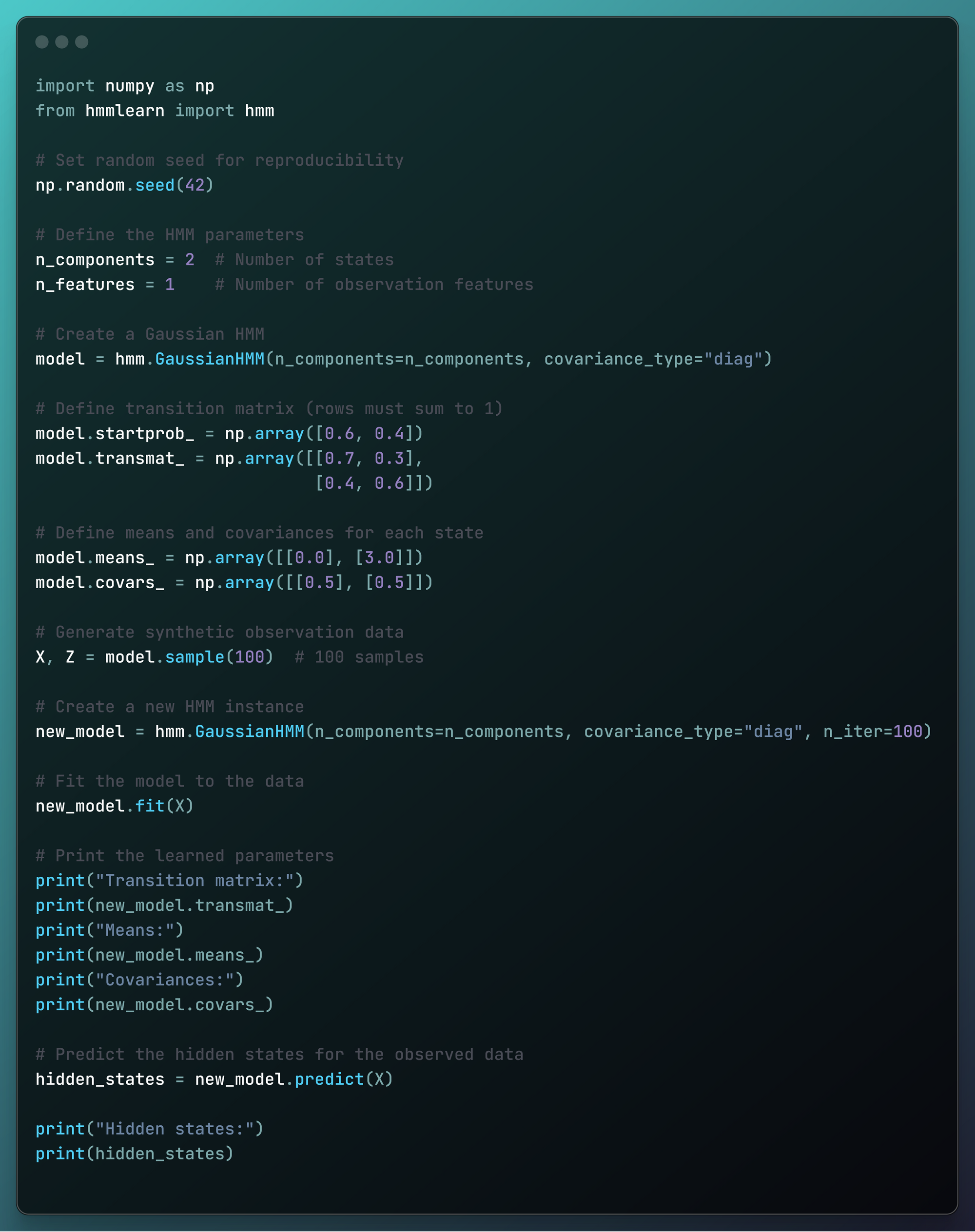
Now let’s break the code down block by block:
Import libraries and set random seed:
import numpy as np
from hmmlearn import hmm

np.random.seed(42)

In this block of code, we imported two Python libraries:
Next we defined a random seed with the NumPy library. A random seed is a value used to start a pseudorandom number generator.
With a fixed random seed, we can ensure that the sequence of pseudorandom numbers generated is always the same. This allows us to duplicate experiments and verify results.
The specific value of the seed doesn’t matter as long as it remains consistent.
Define the HMM parameters and create a Gaussian HMM:
n_components = 2  # Number of states
n_features = 1    # Number of observation features

model = hmm.GaussianHMM(n_components=n_components, covariance_type="diag")

In this code block, we created an HMM with two hidden states and a single observed variable.
covariance_type "diag" means the matrices that represent covariance (how two variables change together) are diagonal. In other words, each row and column is assumed to be independent of the others.
This implies that the probability distributions of each row and column are independent of each other.
But there is still something strange when we defined the hidden Markov chain:
What does “Gaussian“ mean?
This is a very big topic in statistics, but in a few words, Markov chains can only be created when we specify the transition probabilities (chances of moving from one state to another in a Markov chain) and an initial probability distribution.
A Gaussian HMM assumes events are initially modeled by a Gaussian distribution, also called a normal distribution!
And recall, we have already seen before what a normal distribution is.
Here is it again:

From a normal distribution and other components, we can create a hidden Markov chain. And hidden Markov chains serve as a foundation for systems that affect millions of lives.
Define transition matrix, means, and covariances for each state:
model.startprob_ = np.array([0.6, 0.4])
model.transmat_ = np.array([[0.7, 0.3],
                            [0.4, 0.6]])

model.means_ = np.array([[0.0], [3.0]])
model.covars_ = np.array([[0.5], [0.5]])

model.startprob_ = np.array([0.6, 0.4])
This line sets the initial state probabilities for a Hidden Markov Model (HMM). It points out that there is a 60% probability of starting in state 0 and a 40% probability of starting in state 1.
model.transmat_ = np.array([[0.7, 0.3], [0.4, 0.6]])
This line of code sets the state transition probability matrix for the HMM.
The matrix specifies the probabilities of moving from one state to another:
From state 0, there is a 70% chance of staying in state 0 and a 30% chance of transitioning to state 1.
From state 1, there is a 40% chance of transitioning to state 0 and a 60% chance of staying in state 1.
model.means_ = np.array([[0.0], [3.0]])
This line sets the mean values for the observation distributions in each state.
It indicates that the observations are normally distributed with a mean of 0.0 in state 0 and a mean of 3.0 in state 1.
model.covars_ = np.array([[0.5], [0.5]])
This line sets the covariance values for the observation distributions in each state.
It specifies that the variance (covariance in this 1-dimensional case) of the observations is 0.5 for both state 0 and state 1.
Create data, new HMM instance, and fit the model with the data:
X, Z = model.sample(100)  # 100 samples

new_model = hmm.GaussianHMM(n_components=n_components, covariance_type="diag", n_iter=100)

new_model.fit(X)

print("Transition matrix:")
print(new_model.transmat_)
print("Means:")
print(new_model.means_)
print("Covariances:")
print(new_model.covars_)

In this code, we created a model with 100 samples, iterated it 100 times, and printed the new state transition matrix, means, and covariances.
In other words, we:
Generated 100 samples from the original model
Fitted a new HMM to these samples.
Printed the learned parameters of this new model.
What do X and Z mean here?
X means the observed data samples generated by the original model, while Z means the hidden state sequences corresponding to the observed data samples generated by the original model.
The transition matrix prints out:
[[0.8100804  0.1899196 ]
 [0.49398918 0.50601082]]
Which means that the model tends to stay in state 0 and has nearly equal chances of switching or staying when in state 1.
The means print out:
[[0.01577373]
 [3.06245496]]
Which means that the average observed value is approximately 0.016 in state 0 and 3.062 in state 1.
The covariances print out:
[[[0.41987084]]
 [[0.53146802]]]
Which means that the observed values vary by about 0.420 in state 0 and 0.531 in state 1.
This way, we may never know the exact values of the states, but we know their average observed value and how they vary and tend to change with each other.
Predict the hidden states for the observed data:
hidden_states = new_model.predict(X)

print("Hidden states:")
print(hidden_states)

In this code, based on the X observed data samples, we predicted the new states of the Markov model.
The hidden states print out:
[0 0 0 1 0 0 0 0 0 0 0 0 0 0 0 0 0 0 0 0 1 0 1 1 0 0 1 1 0 1 1 0 1 0 0 0 1
 1 1 1 1 0 0 0 1 1 0 0 1 1 1 1 0 0 0 0 0 0 0 1 1 0 0 0 0 0 0 0 0 1 0 0 0 0
 0 0 0 0 0 0 0 0 1 1 0 0 1 0 0 0 0 0 0 0 0 1 1 0 0 0]
Which means that the hidden states switch between state 0 and state 1, showing how the system changes states over time.
Applications in AI and Control Theory: Making Decisions Under Uncertainty

I have been giving you a high-level overview of the field of probabilities and statistics. As I explained before, I wanted to make the explanations simple to understand.
As someone with a bachelor's degree in electrical and computer engineering, I can assure you that while this chapter seems simple, in probabilities and statistics, things can get very complicated very quickly.
Many more concepts like:
p-values
Advanced Monte Carlo methods
Bayesian networks
Statistical hypotheses
Are not as straightforward as the ideas I’ve just told you about.
But as it is, probability and statistics are the starting points for making decisions where uncertainty exists in AI and control theory.
For example, the Bayes’ theorem, besides being the foundation of the Kalman filter, is also the foundation of many probabilistic models in the field of AI. Probabilistic models are usually used in quant firms and banks to model risk.
In control theory, probabilities and statistics are widely used to design robust control systems (as is the case with Kalman filters).
So as you can see, the application of probabilities and statistics, as with calculus and linear algebra, is the foundation for many tools that impact millions of lives and move billions of dollars in the global economy.
Chapter 7: Optimization Theory - Teaching Machines to Improve

This is the most advanced math chapter of the book. To truly understand it, it’s very important that you’ve first read the other chapters first.
We’re going to examine a few machine learning methods, and I’ll show you some recipes of how machine learning is just the use of linear algebra, calculus, probabilities and statistics, and optimization theory.
Just like making a cake!
What is Optimization Theory?
In AI, optimization theory is responsible for the algorithms that optimize data-driven AI models.
Often, big companies invest millions in research to create or refine algorithms that make training AI models faster.
This way, companies save far more money than the upfront research costs when scaling to train multiple large AI models.
It is thanks to optimization theory that deep learning was able to scale efficiently, eventually leading to the creation of ChatGPT and many other large language models.
But why is that?
In all data-driven machine learning models, there is a learning phase that has to happen. That is, there’s a period where the algorithms make predictions that are not correct and then need to change some parameters to make sure the next predictions are correct – or at least closer to being correct.
Without optimization, machine learning algorithms don't get anywhere on their learning path to the right solution. Without optimization, they spend too much time on a learning path that won’t increase their ability to predict things the right way.
So, let’s start learning!
Why Optimization Drives Learning in AI

Optimization theory is the mathematical foundation that allows algorithms to improve their performance over many iterations.
When we combine an algorithm with a path to change its parameters to meet a certain objective (done with an optimization method), it’s called a machine learning algorithm.
This learning process always involves minimizing or maximizing a certain objective. For example, for many machine learning algorithms, the main objective is to minimize errors. To do this, over many iterations, the optimization methods "tells" the internal components of an algorithm what to change after receiving feedback on how well it’s performing.
It’s like someone first learning how to drive a car. The first few times, it may be complicated. But after a while and some practice, the driver learns how to drive properly and not make the same mistakes they once did in the past with the help of the instructor.
The same applies to optimization methods when optimizing algorithms.
Types of Optimization Theory Methods in ML and Deep Learning
The field of optimization theory is huge! Just as with many fields of mathematics, it is constantly growing every year.
But for the purposes of this book, there are three main categories of optimization methods:
- First-Order Methods
These are the most used in deep learning and in all LLM models like Gemini, Grok, and others.
They are called first-order methods because they all use the first derivative of functions. The first derivative of a function measures how much a function's output changes when its input changes very little. The most widely used in deep learning are advanced variants of gradient descent.
While there are many variants, here are some popular examples:
Standard batch gradient descent
Stochastic gradient descent
Mini-batch gradient descent
RMSprop
Adam
In this chapter, we will look in depth at one of these methods called Adam (below).
- Second-Order Methods
They are called second-order methods because they use information from second derivatives for better updates. There are many methods, like:
BFGS
L-BFGS
Newton's method
But these are not often used in machine and deep learning. While they optimize with fewer iterations, for the type of optimization problems algorithms in AI create (high-dimensional problems), they’re very computationally expensive.
So they’re not widely used like first-order optimization methods.
- Zeroth-Order and Other Methods
These methods do not require derivatives to optimize algorithms. Some examples of algorithms where derivatives are not used are:
Genetic algorithms
Dynamic programming algorithms
Particle swarm optimization methods
The problem with these algorithms is that they are often very slow for many variables.
But in certain AI contexts, they can help optimize the architecture of deep learning models to improve AI models from an architectural point of view (instead of a parameter point of view).
How does optimization theory connect with linear algebra, calculus, and probability and statistics?
Essentially:
Calculus teaches you derivatives, which help you understand optimization theory.
Linear algebra teaches you matrices, which help you understand how different states relate and transform.
Probability and statistics teach you concepts like covariance and correlation, which help you understand how variables are connected with each other.
This way, with linear algebra and probability and statistics, you gain the knowledge necessary to understand the algorithms. With calculus you gain the basis to understand optimization theory and how it changes certain parameters of the fundamental algorithms to minimize/maximize a certain objective.
Simple Optimization Techniques: How Machines Learn Step by Step

Now, we’re going to see examples of machine learning algorithms used for optimization and deconstruct them so that you can understand how these areas of mathematics apply to them.
In each example, I will explain their main idea with an analogy as well as how each math area is used in each algorithm.
Linear Regression
Imagine that you are solving a puzzle. To complete the puzzle, you need to arrange the pieces in the right design/order.
The same idea applies to linear regression.
We have matrices (linear algebra) that represent the parameters of the linear regression model and the data that flow into it.
And we can see over time how well the line is fitting the numbers, as well as its error (probabilities and statistics).
To find the best line for the linear regression, we need to know how much the parameters of the model need to change (calculus) and actually apply that change to the parameters (optimization theory).
This way, calculus tells us which direction to change the parameters, and optimization theory tells us how much to actually change them.

Let’s see how to code the linear regression above:
import numpy as np

np.random.seed(42)
X = np.linspace(0, 10, 50)
y_true = 3 * X + 2
noise = np.random.normal(0, 2, 50)
y = y_true + noise

w = 0.1
b = 0.5
learning_rate = 0.01
iterations = [0, 1, 2, 3, 4, 5]
saved_states = []

for epoch in range(max(iterations) + 1):
    y_pred = w * X + b
    error = np.mean((y - y_pred) ** 2)

    if epoch in iterations:
        saved_states.append({
            'epoch': epoch,
            'w': w,
            'b': b,
            'y_pred': y_pred.copy(),
            'error': error
        })

    dw = -2 * np.mean(X * (y - y_pred))
    db = -2 * np.mean(y - y_pred)

    w = w - learning_rate * dw
    b = b - learning_rate * db

Let’s see the code block by block:
Import library:
import numpy as np

For this problem, we’ll import one of the most used Python libraries: NumPy (which we’ve worked with earlier in the book).
Create data points:
np.random.seed(42)
X = np.linspace(0, 10, 50)
y_true = 3 * X + 2
noise = np.random.normal(0, 2, 50)
y = y_true + noise

In this code, we define a base line that will help in generating the data points:

X = np.linspace(0, 10, 50)
y_true = 3 * X + 2
After this green line has been created, we will add noise to it to create the data points:

noise = np.random.normal(0, 2, 50)
y = y_true + noise
This is how we defined the data points for the line dataset.
Initializing linear regression parameters and others:
w = 0.1
b = 0.5
learning_rate = 0.01
iterations = [0, 1, 2, 3, 4, 5]
saved_states = []

In this block of code, we initialize:
Linear regression parameters: Weight to be 0.1 and bias to be 0.5
One hyperparameter: Learning rate
How many iterations we are going to use to improve the linear regression
An array called saved_states to store values to later create graphs
This way, we start with this red line:

Making the linear regression learn with the data:
for epoch in range(max(iterations) + 1):
    y_pred = w * X + b
    error = np.mean((y - y_pred) ** 2)

    if epoch in iterations:
        saved_states.append({
            'epoch': epoch,
            'w': w,
            'b': b,
            'y_pred': y_pred.copy(),
            'error': error
        })

    dw = -2 * np.mean(X * (y - y_pred))
    db = -2 * np.mean(y - y_pred)

    w = w - learning_rate * dw
    b = b - learning_rate * db

It may appear complicated, but let’s see in smaller blocks:
- For loop
for epoch in range(max(iterations) + 1):
- Making an prediction and seeing its error
y_pred = w * X + b
error = np.mean((y - y_pred) ** 2)
In this block of the code, we find the values predicted for the current parameters and see its error from the real values.
- Saving current iteration values for future statistics
if epoch in iterations:
     saved_states.append({
         'epoch': epoch,
         'w': w,
         'b': b,
         'y_pred': y_pred.copy(),
         'error': error
     })
Here we are juts storing in the saved_states array the values of the current iteration to later compute images.
- Finding the gradients
dw = -2 * np.mean(X * (y - y_pred))
db = -2 * np.mean(y - y_pred)
In this block of code, we find the gradients values for the current prediction.
In other words, for the weight and bias, we find out how much they need to change in order to approximate better the values of the parameters to the data points.
- Updating the parameters values
w = w - learning_rate * dw
b = b - learning_rate * db
Finally, we update the weight and the bias with the new values so that the line better approximates the data points:

Neural Networks
The same puzzle idea applies to neural networks. Neural networks are algorithmic models inspired by the brain that learn patterns from data. They are part of a machine learning field called deep learning, which uses neural networks to learn complex patterns.
Neural networks are important because they power modern AI applications like:
Image recognition
Language translation
Chatbots
For example, ChatGPT means Chat Generative Pre-trained Transformer. A transformer is an architecture of neural networks.
If you understand neural networks, you’ll understand the foundations that make ChatGPT work.
We have matrices (linear algebra) that represent the parameters of the neural network model and the data that flow into it.
And we can know over time how well the neural network model is converging to the dataset, fitting the numbers, and see its error (probabilities and statistics).
Calculus will tell us in which direction the parameters of the neural network need to change.
Optimization theory will tell us how much they need to change.
For example, this is a neural network:

This model has in total 13 parameters:
It has 10 lines(connections between circles). These are called weights.
It has 2 circles in the hidden layer and 1 in the output layer. Each circle has one bias.
Big question:
Imagine you work in a bank. You are in charge of deciding who gets credit cards or not. For that, you create the neural network above that takes 4 inputs:
Income
Credit score
Debt ratio
Bankruptcy history
With this neural network well optimized, you can figure it out!
Very simply, without going into things like activation functions, the network processes the 4 inputs through its weights and biases.
Each connection multiplies the input by its weight. After that, each node adds its bias.
The final output is a number between 0 and 1:
Numbers close to 0 mean "Not approved"
Numbers close to 1 mean "Approved"
For example, a high income figure, a good credit score, and no bankruptcy history data flow through the neural networks and produce 0.92. This means that it should be approved.
But a low income figure with a history of bankruptcy may produce 0.15, which results in a not approved.
In reality, bank systems and others have neural networks that take far more well-chosen parameters and decide this automatically.
This is precisely how AI can be used for credit approval.
But a question remains: What is the best way to know how much the parameters need to change?
In the next part, we are going to see the most famous optimization theory algorithm that will help us decide that.
What is Adam? The Most Popular Way AI Models Finds the Best Learning Path

To optimize neural network based AI models, one of the most popular methods is called Adam, which means Adaptive Moment Estimation.
The paper that introduced the method is one of the most influential in the 21st century in machine learning, with thousands of citations. As with all ideas in non-symbolic AI, Adam is a mixture of different math concepts.
It's composed of the ideas of two other optimization methods:
Momentum Gradient Descent: Accumulates velocity from previous gradients to move faster in consistent directions
Root Mean Square Propagation (RMSProp): Adapts learning rates based on recent gradient magnitudes
Let's understand them with an analogy.
Imagine that you are riding a bicycle down a mountain little by little. You already know the direction thanks to calculus.
But how do you descend safely without losing control or going too slowly?
First, you need to build up speed gradually using past momentum. This is one of the main ideas of momentum gradient descent.
It's also important that you adjust your speed based on the terrain's elevation. This is the main idea of RMSProp.
This way, you can safely accelerate and brake appropriately.
When optimizing a model with Adam, this is the same concept. With Adam, we want to optimize a model in a fast and stable way.
The momentum gradient descent ensures the fast part, and the RMSProp ensures the secure part.
Nowadays, for LLMs, which once again are just very big neural network models, a variant of Adam called AdamW is more often used.
Now, let's build a code example of using Adam.
Code example:
Using Adam, we are going to optimize this neural network based on fake data.

It will take 4 features:
Income
Credit score
Debt ratio
Bankruptcy history
And it will tell us if we should or should not approve credit for a given person.
Also, since this book is an introduction to the math of AI, I will not, in this code example, discuss hyperparameter optimization, regularization techniques, and other more advanced topics and good practices.
I want to show why this neural network fails with this data and explain the importance of using great data.
Here is the whole code (and we’ll see each part more in-depth below):
import torch
import torch.nn as nn
import torch.optim as optim
from torch.utils.data import TensorDataset, DataLoader, random_split
import pytorch_lightning as pl
import matplotlib.pyplot as plt

torch.manual_seed(42)
x = torch.randn(10000, 4)
y = torch.randint(0, 2, (10000, 1)).float()
dataset = TensorDataset(x, y)

train_size = int(0.8 * len(dataset))
val_size = len(dataset) - train_size
train_dataset, val_dataset = random_split(dataset, [train_size, val_size])

train_loader = DataLoader(train_dataset, batch_size=32, shuffle=True)
val_loader = DataLoader(val_dataset, batch_size=32)

class CreditApprovalNet(pl.LightningModule):
    def __init__(self):
        super().__init__()
        self.hidden = nn.Linear(4, 2)
        self.relu = nn.ReLU()
        self.output = nn.Linear(2, 1)
        self.sigmoid = nn.Sigmoid()
        self.loss_fn = nn.BCELoss()
        self.train_losses = []

    def forward(self, x):
        x = self.relu(self.hidden(x))
        return self.sigmoid(self.output(x))

    def training_step(self, batch, batch_idx):
        x, y = batch
        y_pred = self(x)
        loss = self.loss_fn(y_pred, y)
        self.log('train_loss', loss)
        self.train_losses.append(loss.item())
        return loss

    def configure_optimizers(self):
        return optim.Adam(self.parameters(), lr=0.0001)

model = CreditApprovalNet()
trainer = pl.Trainer(max_epochs=100, logger=False, enable_checkpointing=False)
trainer.fit(model, train_loader, val_loader)

#
plt.plot(model.train_losses)
plt.xlabel('Training Step')
plt.ylabel('Loss')
plt.title('Credit Approval Training')
plt.grid(True, alpha=0.3)
plt.show()

Now let’s break it down:
Importing libraries:
import torch
import torch.nn as nn
import torch.optim as optim
from torch.utils.data import TensorDataset, DataLoader, random_split
import pytorch_lightning as pl
import matplotlib.pyplot as plt

In this block of code, we are importing code from 3 Python libraries:
PyTorch: One of the most popular python libraries to create new AI models in AI research
PyTorch Lightning: A PyTorch wrapper that organizes training code and handles repetitive tasks automatically
Matplotlib: One of the most popular python libraries to make graphs from data
Creating data:
torch.manual_seed(42)
x = torch.randn(10000, 4)
y = torch.randint(0, 2, (10000, 1)).float()
dataset = TensorDataset(x, y)

In this part, we define a seed to make the random numbers reproducible. In other words, when we run the code many times, the same random numbers will be generated.
Next, we will create 10,000 applications for credit with 4 features in X and their approval decisions in y. After that, we unify everything in the dataset variable.
We’ll use TensorDataset because it allows us to have the 4 features and the target paired together. This way, the data does not get mixed up during training.
Dividing data:
train_size = int(0.8 * len(dataset))
val_size = len(dataset) - train_size
train_dataset, val_dataset = random_split(dataset, [train_size, val_size])

In this block of code, we divide the data into a training dataset and a validation dataset.
This way, we have one dataset that’s being used to train and find the parameters while comparing results with the validation dataset.
As we can see, 80% of the data will be training data, and 20% of the data will be validation data.
Loading data:
train_loader = DataLoader(train_dataset, batch_size=32, shuffle=True)
val_loader = DataLoader(val_dataset, batch_size=32)

Here, we load the data into data loaders for the AI model to use.
This way, we have the data automatically split into small batches and shuffled. So instead of processing all 10,000 data points, the model will be trained on one batch, improved, then another batch, then improved again, and so forth. That makes training go faster.
Creating AI model and training process:
class CreditApprovalNet(pl.LightningModule):
    def __init__(self):
        super().__init__()
        self.hidden = nn.Linear(4, 2)
        self.relu = nn.ReLU()
        self.output = nn.Linear(2, 1)
        self.sigmoid = nn.Sigmoid()
        self.loss_fn = nn.BCELoss()
        self.train_losses = []

    def forward(self, x):
        x = self.relu(self.hidden(x))
        return self.sigmoid(self.output(x))

    def training_step(self, batch, batch_idx):
        x, y = batch
        y_pred = self(x)
        loss = self.loss_fn(y_pred, y)
        self.log('train_loss', loss)
        self.train_losses.append(loss.item())
        return loss

    def configure_optimizers(self):
        return optim.Adam(self.parameters(), lr=0.0001)

This code block appears to be complicated, but let’s see each method block by block:
- Creating the class with inheritance:
class CreditApprovalNet(pl.LightningModule):
This way, in one line, we can import everything we need to define both the model and how it will be trained.
- init: Builds the model's layers and components:
    def __init__(self):
        super().__init__()
        self.hidden = nn.Linear(4, 2)
        self.relu = nn.ReLU()
        self.output = nn.Linear(2, 1)
        self.sigmoid = nn.Sigmoid()
        self.loss_fn = nn.BCELoss()
        self.train_losses = []
In this section of the code, we are defining the architecture of the AI model.
- forward: Processes input data through the network to make predictions:
    def forward(self, x):
        x = self.relu(self.hidden(x))
        return self.sigmoid(self.output(x))
In this part of the code, we are defining how data will flow in the AI model based on the architecture defined.
- training_step: Calculates loss for each batch during training:
    def training_step(self, batch, batch_idx):
        x, y = batch
        y_pred = self(x)
        loss = self.loss_fn(y_pred, y)
        self.log('train_loss', loss)
        self.train_losses.append(loss.item())
        return loss
Here, we are defining how the model will be trained. In other words, how we will find the best parameters for the model to predict well.
- configure_optimizers: Sets the Adam optimizer with learning rate:
    def configure_optimizers(self):
        return optim.Adam(self.parameters(), lr=0.0001)
Finally, here we are defining what optimizer we are going to use to, step by step, improve the AI model parameters.
Training AI model:
model = CreditApprovalNet()
trainer = pl.Trainer(max_epochs=100, logger=False, enable_checkpointing=False)
trainer.fit(model, train_loader, val_loader)

In this block of code:
We create the neural network model in the first line
In the 2nd and 3rd line, we prepare the training settings and train the model for 100 epochs
This way, in the command line, this appears:

The PyTorch code is essentially telling us the number of parameters in the AI model!
Seeing results and understanding why they are not good:
plt.plot(model.train_losses)
plt.xlabel('Training Step')
plt.ylabel('Loss')
plt.title('Credit Approval Training')
plt.grid(True, alpha=0.3)
plt.show()

Using the Matplotlib library, we plot the results:

The AI model is not converging.
We can see that because the loss is nearly 0.7 (70%) over time.
The main reason the model is not converging well is that there is little to no relationship between the 4 features and the target variable.
In other words, we do not have good data.
The code works perfectly, but this shows the most important rule in machine learning: when we create an AI model, the MOST IMPORTANT thing is data.
It does not matter if you use a simple linear regression or a neural network based on transformers or whatever. If you do not have high quality data, the model is not going to perform well.
Even if we use a good optimizer, like Adam, it will not solve the data problem.
Next steps: Common beginner mistakes
I also wrote this exact code example to show you something very important: neural networks are not always the best models to use.
This is a very common beginner mistake. You may start with neural networks for everything, when often machine learning methods with little data preprocessing do the job well.
For this type of problem, the solution is to first try machine learning methods instead of going to neural networks.
There are many reasons for this, but the main ones are:
Machine learning methods are simpler and often quicker to train than neural networks
Machine learning methods are simpler to understand how they make decisions. In other words, we can understand how the machine learning model thought to make a prediction.
With computational learning, we can guess with certain machine learning models how well they will predict in the future and provide theoretical guarantees about their performance.
Another common mistake is not dividing the data.
To simplify, I created only a training and validation division of the data
In a serious project, you should always divide it into 3 parts: training, validation, and testing.
With training, you create the model. With validation, you test the model based on the data it was trained on. With the test dataset part, you compare if the loss of the model is similar to the validation or different. If they are very different, it means that the AI model converged to the validation dataset but not the test dataset.
I challenge you to think further about how you could improve this code and to try to make the synthetic data more correlated in order to improve its quality.
Applications in AI and Control Theory of Optimization Theory

Optimization theory serves as the engine behind AI and control systems that shape our lives.
From unlocking your phone with facial recognition to autopilot systems guiding planes, optimization algorithms are constantly at work.
When you ask ChatGPT a question, optimization theory determines the values of billions of parameters during training.
The same is true for all other LLMs like Gemini, Claude, Grok, DeepSeek, and others. All of them contain millions and millions of parameters. The only way to find the best combination of the parameters to achieve a certain objective is with optimization theory.
In control theory, many systems like Model Predictive Control (MPC) and adaptive control systems only work thanks to optimization methods that balance how internal components of the control system should work together
Beyond training neural networks and controlling physical systems, optimization powers recommendation systems, resource allocation, and so many other systems.
Some examples are:
Netflix movie recommendation system
Spotify's song suggestion system
Google systems to reduce data center cooling costs
Quantitative trading firms high-frequency trading systems
To end this final chapter, I’ll share this:
It is optimization theory that makes math models into AI models that impact the lives of millions worldwide.
Conclusion: Where Mathematics and AI Meet

When ancient civilizations first carved numbers into clay tablets, they likely didn’t imagine that these symbols would one day allow humanity to create the scientific, technological, and medical marvels we have today.
Yet here we are.
We’re in an era where mathematical ideas developed over many centuries – even millennia – have converged to create artificial intelligence.
Throughout this book, we've traced a path from the most basic math concepts to the cutting edge of AI. We have seen how:
Matrices compress complex systems into simple forms
Derivatives measure change
Probability helps us navigate uncertainty
Optimization guides algorithms toward better decisions to learn faster.
We’ve also learned how each math field has helped create tools that are responsible for many of the things we take for granted today.
Mathematics is the Foundation of AI

Always remember this: AI is not pure magic or a "being" we don't understand. It’s just the combination of many math ideas working very well together.
When you ask a question of ChatGPT or any other LLM, it generates a response. And in the process of generating that response, there are millions of matrix multiplications happening in seconds.
Or, for example, when a self-driving car decides to stop moving because it’s coming up to a crosswalk, there are a lot of math computations (related to calculus and probability and statistics) working very fast to ensure safety.
The great thing about mathematics is that it’s a common, standard language of logic. No matter the backgrounds of people or where they were born, a derivative will always be a derivative, and the same thing goes for key AI concepts.
This way, scientists and engineers worldwide can improve each other's work because everyone understands the same language.
The Future: On Device AI and the Democratization of AI

One shift happening now is the move toward edge AI. That is, AI that runs locally on your phone, computer, and really in all your devices (rather than in distant data centers).
This way, privacy is guaranteed because it runs locally. Waiting times for AI models decrease because no data needs to be sent. AI can be used offline, and costs decrease.
And what about the massive data centers being built all over the world? Those will be used for more products that will help improve the lives of millions of people.
As AI becomes more local and more processing power is freed up from big data centers, new AI innovations will appear, and more benefits will come.
The same way that in the past century every computer got its own networking chip, every device will have (and in some cases, already has) AI accelerators.
And much of it will be thanks to the math you learned in this book.
Final Reflections
Isaac Newton wrote, "If I have seen further, it is by standing on the shoulders of giants."
Every algorithm you use, every model you train, and every new theorem you learn stands on centuries of mathematical progress. You now stand on those same shoulders of these giants!
Thank you for reading, and happy learning.
Here’s the full book GitHub repository with all the code.
Acknowledgements
First and foremost, I would like to thank Guilherme Mendes, currently a Master’s student in Electrical and Computer Engineering at NOVA University, specializing in Control Theory, for reviewing the mathematical and technical details of the 1st version of this book.
I am also grateful to the organizations that gave me opportunities to grow:
A special thank you goes to the freeCodeCamp editorial team**,** especially Abigail Rennemeyer, for their patience and for reviewing every chapter of this book.
I would also like to thank all the professors at NOVA FCT who have taught and guided me throughout my academic journey, especially those from the Department of Electrical and Computer Engineering.
About the Author
Email: monteiro.t@northeastern.edu
My name is Tiago Monteiro, and I’m now pursuing a master's degree in Artificial Intelligence at Northeastern University in the Silicon Valley Campus (San Jose) on a merit-based scholarship.
I’m not from the United States. I am a Portuguese national, born and raised in the district of Lisbon.
In Portugal, I completed a bachelor's degree in electrical and computer engineering at NOVA University, one of Portugal's best universities.
I have authored over 20 articles for freeCodeCamp, which have accumulated more than 240,000 views over the years, and completed the Deep Learning Specialization from DeepLearningAI, taught by Andrew Ng.
Also, I had the privilege of participating in the winter 2025 batch of the renowned Silicon Valley Fellowship program.
Why did I choose electrical and computer engineering?
After finishing the Portuguese national math exam in 12th grade, I chose Electrical and Computer Engineering (ECE) to challenge myself and learn new math on my own.
The ECE degree combined:
Advanced Mathematics
Programming (from Assembly to Python)
Physics (classical mechanics, electromagnetism)
What did I gain exactly?
I mastered the skills needed to quickly understand AI research, particularly after completing Andrew Ng's Deep Learning Specialization.
In Portugal, I also studied advanced STEM areas including, for example:
Partial Differential Equations for modeling real-world phenomena
Harmonic analysis (Fourier/Laplace transforms) for signal processing and alternative problem perspectives
Complex analysis involving derivatives and integrals in the complex domain
Numerical methods for approximating mathematical solutions computationally
Signal/control theory for ensuring system stability in dynamic environments
Physics classes in classical mechanics and electromagnetism fundamentals
While not directly applied to AI, these studies enhanced my systems thinking and ability to independently learn complex STEM concepts.