By Tanveer Sayyed
And using a “soft” method to impute the same.
This post focuses more on a conceptual level rather than coding skills and is divided into two parts. Part-I describes the problems with missing values and when and why should we use mean/median/mode. Part-II repudiates Part-I and argues why we should use none of them and use the soft method instead— random but proportional representation.
 _Photo by [Pexels](https://www.pexels.com/@rakicevic-nenad-233369?utm_content=attributionCopyText&utm_medium=referral&utm_source=pexels" rel="noopener" target="_blank" title="">Rakicevic Nenad from <a href="https://www.pexels.com/photo/silhouette-photo-of-man-throw-paper-plane-1262304/?utm_content=attributionCopyText&utm_medium=referral&utm_source=pexels" rel="noopener" target="blank" title=")
Part-I: Why do we remove missing values? When to use mean, median, mode? And Why?
The problem with missing data is that there is no fixed way of dealing with them, and the problem is universal. Missing values affect our performance and predictive capacity. They have the potential to change all our statistical parameters. The way they interact with outliers once again affects our statistics. Conclusions can thus be misleading.
The different missing values can be:
- NaN
- None
- “Null”
- “missing”
- “not available”
- “NA”
While the last four are string values, pandas by default identify NaN(no assigned number) and None. However, both are not the same; the code snippet below shows why.
The problem is that if we do not remove the NaNs then, we are in for double jeopardy. Firstly we already are suffering from loss of true data and secondly if not handled with care NaNs start ‘devouring’ our true data and might get propagated throughout the data-set as we proceed. Let's instantiate two series and see.
Now let’s see what happens when we perform certain operations on those lists.
We can see how true data (integers 1, 2) were lost while performing operations (Out: 21, 22). Another thing to note is conflicting results in the in-built python method and the series method due to the presence of NaNs (Out: 23, 24).
Now let’s create a data-frame which has all the missing values stated above as well as a garbage value(‘#$%’). We’ll remove missing values by wrangling with this tiny toy data-set.
The data-frame has one complete row(i1) and one complete column(c2) filled with only NaNs. Other missing value identifiers have also been deliberately scattered.
Above we can see that the last term in c3 should be “True”(for “not available”). To make it so we’ll have to read the data-frame again. This time we’ll force pandas to identify “missing”/“not available” /”NA” as NaNs.
All missing values have been identified, shall we get rid of them by dropping them altogether?
Looks like we lost all the values! The .dropna() deletes the complete row(index) even if a “single” value is missing. Hence .dropna() comes with the price of losing data which may be valuable.
How to proceed?
Now one may presume imputing all missing values with — zero. But there is a fundamental problem with this approach: the sanctity/veracity of our data is lost, as in the real world a missing term can take ANY value. But we are forcing it to take only one rigid value, i.e. 0.
The official document of sklearn mentions: (emphasis mine)
… infer them(missing values) from the known part of the data.
So what should we do now? A better option is to use mean as it at least is a better “representative” of a feature than zero. Why? Because for continuous/numeric features no matter how many times we add mean, it still gets conserved. Here is how:
Three numbers — 2, 6, 7 — have, mean = (2 + 6 + 7)/3 = 5
Assuming this list has an infinite number of missing values, lets impute it with mean: — 2, 6, 7, 5, 5, 5, 5….. The mean will remain 5 no matter how many times we add it!
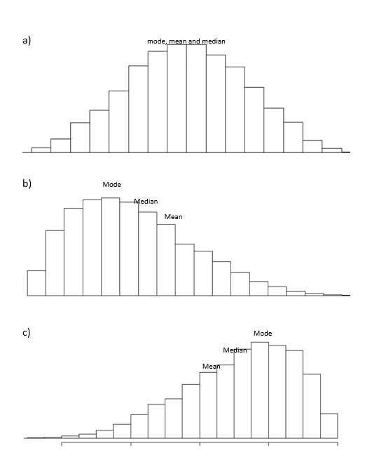
But there are problems with mean. Firstly it is heavily influenced by outliers, mean(2 + 6 + 7+ 55) = 17.5! Secondly, although it does ‘represent’ a feature, it is also the worst in reflecting central tendency of a normal data(see below bullets b & c [respectively for right skewed and left skewed data]).
 _[commons.wikimedia](https://commons.wikimedia.org/wiki/File:Measures_of_Central_Tendency.png" rel="noopener" target="blank" title=")
As we can clearly observe in bullets b & c, the mode best reflects the central tendency. Mode is the most frequent value in our data set. But when it comes to continuous data then mode can create ambiguities. There might be more than one mode or (rarely)none at all if none of the values are repeated. Mode is thus used to impute missing values in columns which are categorical in nature.
After mode, it is the median that reflects the central tendency the best. Which implies that for continuous data, the use of the median is better than mean! Median is the middle score of data-points when arranged in order. And unlike the mean, the median is not influenced by outliers of the data set — the median of the already arranged numbers (2, 6, 7, 55) is 6.5!
So for categorical data using mode makes more sense and for continuous data the median. So why do we still use mean for continuous data?
Legacy
Previously in the world with no computers, it was easier to calculate the mean than the median. In those times it definitely made sense as re-arranging thousands of entries manually, each time the data-set is updated, and then finding the median was indeed a cumbersome task. But should we continue this legacy, when we have the power of computation at our fingertips, today? No, that would imply under-utilizing our potential.
But again, the rigidity remains, as we are still using a single value — mean/median/mode. We’ll discuss more about this in the next section shortly. For now let’s replace values with mean(in c0), median(in c1) and mode(in c3). Before, let’s deal with the garbage value ‘#$%’ at (‘i2’, ‘c3’).
The respective values are:
We’ll use 3 different methods to replace NaNs.
It looks like we’ll have to drop the c2 column altogether as it contains no data. Note that in the beginning one row and one column were completely filled with NaNs but we were only able to successfully manipulate the rows but not the columns. Dropping c2.
We finally got rid of all the missing values!
Part-II: Random but proportional replacement (RBPR)
 _Photo by [Pexels](https://www.pexels.com/@rakicevic-nenad-233369?utm_content=attributionCopyText&utm_medium=referral&utm_source=pexels" rel="noopener" target="_blank" title="">Rakicevic Nenad from <a href="https://www.pexels.com/photo/silhouette-of-person-holding-glass-mason-jar-1274260/?utm_content=attributionCopyText&utm_medium=referral&utm_source=pexels" rel="noopener" target="blank" title=")
The above methods, I think, can be described as hard imputation approaches, as they rigidly accept only one value. Now let’s focus on a “soft” imputation approach. Soft because it makes use of probabilities. Here we are not forced to pick a single value. We’ll replace NaNs randomly in a ratio which is “proportional” to the population without NaNs (the proportion is calculated using probabilities but with a touch of randomness).
An explanation with an example would be better. Assume a list having 15 elements with one-third data missing:
[1, 1, 1, 1, 2, 2, 2, 2, 3, 3, NaN, NaN, NaN, NaN, NaN] — — — (original)
Now notice in the original list there are sets of 4 ones, 4 twos, 2 threes, and 5 NaNs. Thus the ones & twos are in majority while threes are in minority. Now let's begin by calculating the probabilities and expected values.
- prob(1 occurring in NaNs)
= (no. of 1s)/(population without NaNs)
= 4/10
= 2/5 - Expected value/counts of 1
= (prob) (total no. of NaNs)
= (2 / 5) (5)
= 2
Similarly expected value of prob(2 occurring in NaNs) is 2 and prob(3 occurring in NaNs) is 1 (Note that 2+2+1=5, is equal to the number of NaNs). Thus our list will now look like this:
[1, 1, 1, 1, 2, 2, 2, 2, 3, 3, 1, 1, 2, 2, 3] — — — (_replaced_byproportion)
The ratio of ones, twos, and threes replacing NaNs is thus 2 : 2 : 1. That is when we have ‘nothing’ it is highly likely that ‘ones’ and ‘twos’ form the major part of it than ‘threes’, instead of a single hard mean/mode/median.
If we simply impute NaNs by mean(1.8), then our list looks like:
[1, 1, 1, 1, 2, 2, 2, 2, 3, 3, 1.8, 1.8, 1.8, 1.8, 1.8] — — — (_replaced_bymean)
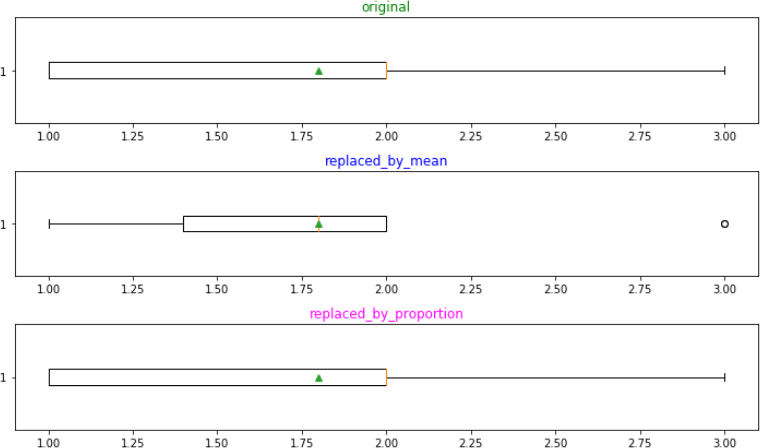
Let’s box-plot these three lists and draw conclusions from the same:
 _[Box-plot code (NaN-12.py)](https://gist.github.com/Vernal-Inertia/e8d95749416b2df6b8f63ee124b7b73b" rel="noopener" target="blank" title=")
First, the list with proportional replacement has far better data distribution than the mean replaced one. Second, observe how mean affects the distribution with ‘3’(a minority): it was originally not an outlier, suddenly turned so in plot-2 but regained its original status in plot-3. This shows that plot-3 distribution is less biased. Third, this approach is also fairer, it gave ‘3’(the minority) a “chance” in the missing values which otherwise it would have never got. The fourth beauty of this approach is that we still have successfully conserved the mean!
Fifth, the distribution (based on probability) ensures, without doubt, that the chances of this method to over-fit a model is definitely lesser than imputing with the hard approach. Sixth, if NaNs are replaced “randomly” then applying a little logic we can easily calculate that there are: 5!/(2!2!1!) = 30, different arrangements (permutations) possible:
… 1, 1, 2, 2, 3],
… 1, 1, 2, 3, 2],
… 1, 1, 3, 2, 2],
… 1, 3, 1, 2, 2],
… 3, 1, 1, 2, 2] and 25 more!
To make this dynamism even clearer and intuitive see this gif with 4 NaNs. Each color represents a different NaN value.

Notice how different arrangements generate different _interaction_s between columns each time we run the code. Per se, we are not ‘generating’ new data here, as we are only resourcefully utilizing the already available data. We are only generating newer and newer interactions. And these fluctuating interactions are the real penalty of NaNs.
Code:
Now let’s code this concept and bound it. The code for dealing with numerical features can be found here and for categorical features here. (I am purposely avoiding displaying the code here as the focus is on the concept, also it would needlessly make the article lengthy. If you do find the code useful and are [algorithmically] greedy enough to optimize it further, I’ll be glad if you revert). How to use the code?
random.seed = 0 np.random.seed = 0# important so that results are reproducible
# The df_original is free of impurities(eg. no '$' or ',' in price # field) and df_original.dtypes are all set.
1. df = df_original.copy()2. Call the CountAll() function given in the code3. categorical list = [all categorical column names in df]4. numerical list = [all numerical column names in df]5. run a for loop to fill NaNs through numerical list, using the Fill_NaNs_Numeric() function6. run a for loop to fill NaNs through categorical list, using the Fill_NaNs_Catigorical() function7. perform a train test split and check for the accuracy(do not specify the random_state)
(After step 7 we require a bit of imputation tuning. Ensuring steps 1-7 are in a single cell, repeatedly run it 15-20 times manually to get an idea of the 'range' of accuracies as it'll keep fluctuating due to randomness. 7th step helps one get an estimate of the limits of accuracies and helps us to boil down to the "best accuracy")
8.("skip" this step if df is extremely huge) run a conditioned while loop again through 1 to 7 this time to directly get our desired(tuned) accuracy.
(One may want to write down and save this 'updated'-df for future use to save oneself from repeating this process).
Here is a complete example, with all the steps just mentioned, on the famous Iris data-set included in sklearn library. 20% values from each column, including the target, have been randomly deleted. Then the NaNs in this data-set is imputed using this approach. By step-7 its easily identifiable that after imputation we can tune our recall at-least ≥ 0.7 for “each” class of the iris plant, and the same is the condition in the 8-th step. After running several times few reports are as follows:
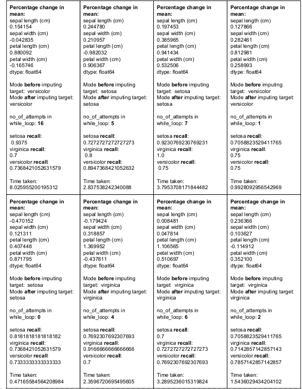 Soft Imputation on Iris Dataset
Next, for a second confirmation, we plot PR-curves post-tuning, this time with a RandomForestClassifier (n_estimators= 100). [the classes are {0 :’setosa’, 1: ‘versicolor’, 2: ‘virginica’}].
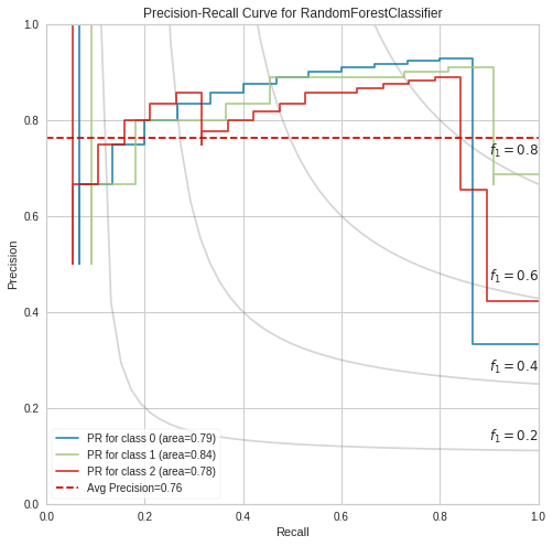 Measuring the RBPR’s quality through the area under the curve
These figures look okay. Now shifting our attention to hard imputation. One of the many classification reports is shown below: [observe the 1s(to be discussed shortly) in precision and recall along with the class imbalance in support]
precision recall f1-score support
setosa 1.00 0.52 0.68 25versicolor 0.45 1.00 0.62 9virginica 0.67 0.73 0.70 11
The law of large numbers
Now lets put to use the law of large numbers using DecisionTreeClassifier to perform 500 iterations, each with a different randomly removed set of values, over the same Iris dataset without tuning the imputations; that is, we skip the tuning stage to “deliberately” obtain the worst soft scores. The code is here. The final comparisons in terms of precision and recall scores, for both hard and soft imputation, are as follows:
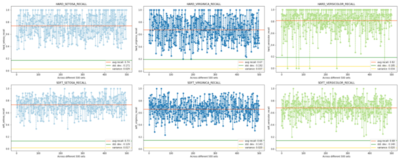 RECALLS
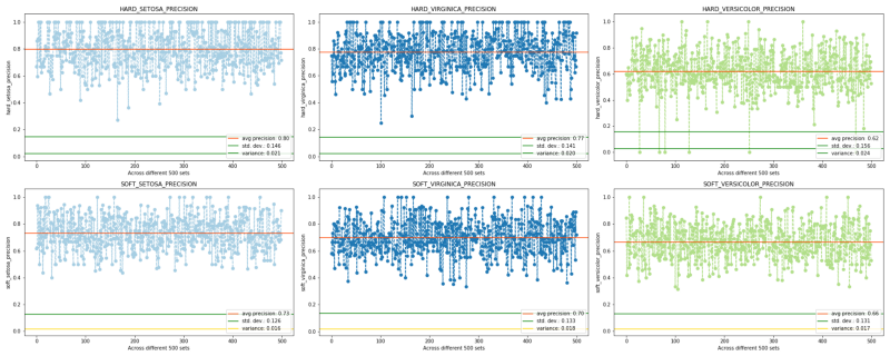 PRECISIONS
Precision and recall come handy mainly when we observe class imbalance. Although initially, we did have a well-balanced target but hard imputing with it with mode made it imbalanced. Observe a large number of hard recalls and hard precisions having value = 1. Here the use of the word “over-fit” would be incorrect as these are test scores not train ones. So the correct way to put would be: the prophetic hard model already knew what to predict, or the use of mode ensured the two scores to overshoot.
Now observe the soft scores. Despite any tuning as well as much fewer values being= 1, the soft scores are still able to catch up/converge with the hard scores (except in two cases — versicolor-recall and stetosa-precision — for obvious reasons where a huge number of prophetic 1s forcefully pull up the average). Also, observe the soft-stetosa-recall (despite the presence of large 1s in the hard counterpart), and, the increased soft-versicolor-precision. The last thing to note is the overall reduction in variation and standard deviation in the soft approach.
For reference the f1 scores and accuracy scores are: (once again note the reduced variation and standard deviation in soft approach)
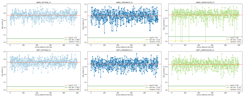 F1-SCORE
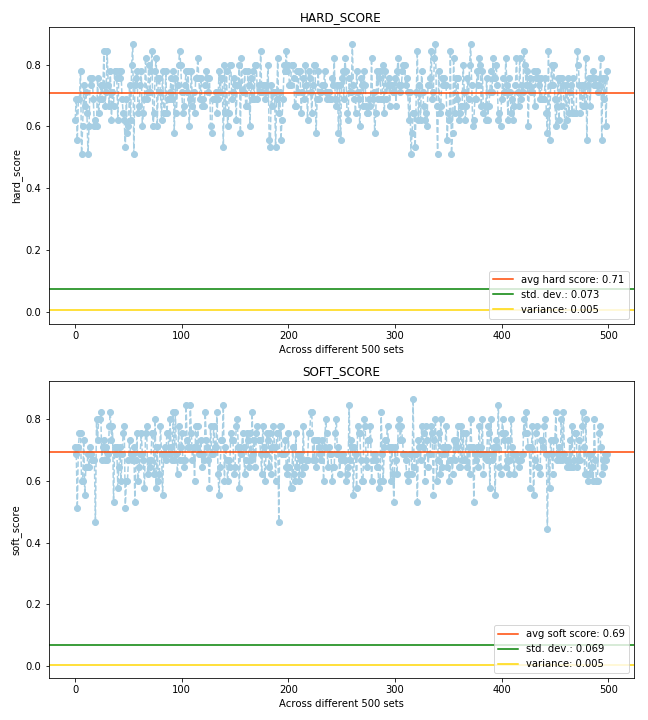 ACCURACY SCORES
Thus we can observe that in the long run, even without soft imputation tuning we have obtained results which match the performance of the hard imputation strategy. Thus after tuning we can obtain even better results.
Conclusion
Why are we doing this? The only reason is to improve our chances of dealing with uncertainty. We never penalize ourselves for missing values! Whenever we find a missing value we simply anchor our ship in the ‘middle’ of the sea falsely presuming that our anchor has successfully fathomed the deepest trench of “uncertainties”. The attempt here is to keep the ship sailing by employing the resources available at hand — the wind speed and direction, the location of stars, the energy of the waves and tides, etc. to get the best ‘diversified’ catch, for a better return.
 Photo by Simon Matzinger from Pexels
(If you identify anything wrong/incorrect, please do respond. Criticism is welcomed).