The Ultimate Guide to the Pandas Library for Data Science in Python

Pandas (which is a portmanteau of "panel data") is one of the most important packages to grasp when you’re starting to learn Python.

The package is known for a very useful data structure called the pandas DataFrame. Pandas also allows Python developers to easily deal with tabular data (like spreadsheets) within a Python script.

This tutorial will teach you the fundamentals of pandas that you can use to build data-driven Python applications today.

Table of Contents

You can skip to a specific section of this pandas tutorial using the table of contents below:

• Introduction to Pandas
• Pandas Series
• Pandas DataFrames
• How to Deal With Missing Data in Pandas DataFrames
• The Pandas groupby Method
• What is the Pandas groupby Feature?
• The Pandas concat Method
• The Pandas merge Method
• The Pandas join Method
• Other Common Operations in Pandas
• Local Data Input and Output (I/O) in Pandas
• Remote Data Input and Output (I/O) in Pandas
• Final Thoughts & Special Offer

Introduction to Pandas

Pandas is a widely-used Python library built on top of NumPy. Much of the rest of this course will be dedicated to learning about pandas and how it is used in the world of finance.

What is Pandas?

Pandas is a Python library created by Wes McKinney, who built pandas to help work with datasets in Python for his work in finance at his place of employment.

According to the library’s website, pandas is “a fast, powerful, flexible and easy to use open source data analysis and manipulation tool, built on top of the Python programming language.”

Pandas stands for ‘panel data’. Note that pandas is typically stylized as an all-lowercase word, although it is considered a best practice to capitalize its first letter at the beginning of sentences.

Pandas is an open source library, which means that anyone can view its source code and make suggestions using pull requests. If you are curious about this, visit the pandas source code repository on GitHub

The Main Benefit of Pandas

Pandas was designed to work with two-dimensional data (similar to Excel spreadsheets). Just as the NumPy library had a built-in data structure called an array with special attributes and methods, the pandas library has a built-in two-dimensional data structure called a DataFrame.

What We Will Learn About Pandas

As we mentioned earlier in this course, advanced Python practitioners will spend much more time working with pandas than they spend working with NumPy.

Over the next several sections, we will cover the following information about the pandas library:

• Pandas Series
• Pandas DataFrames
• How To Deal With Missing Data in Pandas
• How To Merge DataFrames in Pandas
• How To Join DataFrames in Pandas
• How To Concatenate DataFrames in Pandas
• Common Operations in Pandas
• Data Input and Output in Pandas
• How To Save Pandas DataFrames as Excel Files for External Users

Pandas Series

In this section, we’ll be exploring pandas Series, which are a core component of the pandas library for Python programming.

What Are Pandas Series?

Series are a special type of data structure available in the pandas Python library. Pandas Series are similar to NumPy arrays, except that we can give them a named or datetime index instead of just a numerical index.

The Imports You’ll Require To Work With Pandas Series

To work with pandas Series, you’ll need to import both NumPy and pandas, as follows:

import numpy as np

import pandas as pd

For the rest of this section, I will assume that both of those imports have been executed before running any code blocks.

How To Create a Pandas Series

There are a number of different ways to create a pandas Series. We will explore all of them in this section.

First, let’s create a few starter variables - specifically, we’ll create two lists, a NumPy array, and a dictionary.

labels = ['a', 'b', 'c']

my_list = [10, 20, 30]

arr = np.array([10, 20, 30])

d = {'a':10, 'b':20, 'c':30}

The easiest way to create a pandas Series is by passing a vanilla Python list into the pd.Series() method. We do this with the my_list variable below:

pd.Series(my_list)

If you run this in your Jupyter Notebook, you will notice that the output is quite different than it is for a normal Python list:

0    10

1    20

2    30

dtype: int64

The output shown above is clearly designed to present as two columns. The second column is the data from my_list. What is the first column?

One of the key advantages of using pandas Series over NumPy arrays is that they allow for labeling. As you might have guessed, that first column is a column of labels.

We can add labels to a pandas Series using the index argument like this:

pd.Series(my_list, index=labels)

#Remember - we created the 'labels' list earlier in this section

The output of this code is below:

a    10

b    20

c    30

dtype: int64

Why would you want to use labels in a pandas Series? The main advantage is that it allows you to reference an element of the Series using its label instead of its numerical index. To be clear, once labels have been applied to a pandas Series, you can use either its numerical index or its label.

An example of this is below.

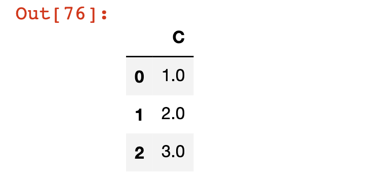
Series = pd.Series(my_list, index=labels)

Series[0]

#Returns 10

Series['a']

#Also returns 10

You might have noticed that the ability to reference an element of a Series using its label is similar to how we can reference the value of a key-value pair in a dictionary. Because of this similarity in how they function, you can also pass in a dictionary to create a pandas Series. We’ll use the d={'a': 10, 'b': 20, 'c': 30} that we created earlier as an example:

pd.Series(d)

This code’s output is:

a    10

b    20

c    30

dtype: int64

It may not yet be clear why we have explored two new data structures (NumPy arrays and pandas Series) that are so similar. In the next section of this section, we’ll explore the main advantage of pandas Series over NumPy arrays.

The Main Advantage of Pandas Series Over NumPy Arrays

While we didn’t encounter it at the time, NumPy arrays are highly limited by one characteristic: every element of a NumPy array must be the same type of data structure. Said differently, NumPy array elements must be all string, or all integers, or all booleans - you get the point.

Pandas Series do not suffer from this limitation. In fact, pandas Series are highly flexible.

As an example, you can pass three of Python’s built-in functions into a pandas Series without getting an error:

pd.Series([sum, print, len])

Here’s the output of that code:

0      <built-in function sum>

1    <built-in function print>

2      <built-in function len>

dtype: object

To be clear, the example above is highly impractical and not something we would ever execute in practice. It is, however, an excellent example of the flexibility of the pandas Series data structure.

Pandas DataFrames

NumPy allows developers to work with both one-dimensional NumPy arrays (sometimes called vectors) and two-dimensional NumPy arrays (sometimes called matrices). We explored pandas Series in the last section, which are similar to one-dimensional NumPy arrays.

In this section, we will dive into pandas DataFrames, which are similar to two-dimensional NumPy arrays - but with much more functionality. DataFrames are the most important data structure in the pandas library, so pay close attention throughout this section.

What Is A Pandas DataFrame?

A pandas DataFrame is a two-dimensional data structure that has labels for both its rows and columns. For those familiar with Microsoft Excel, Google Sheets, or other spreadsheet software, DataFrames are very similar.

Here is an example of a pandas DataFrame being displayed within a Jupyter Notebook.

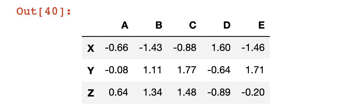
We will now go through the process of recreating this DataFrame step-by-step.

First, you’ll need to import both the NumPy and pandas libraries. We have done this before, but in case you’re unsure, here’s another example of how to do that:

import numpy as np

import pandas as pd

We’ll also need to create lists for the row and column names. We can do this using vanilla Python lists:

rows = ['X','Y','Z']

cols = ['A', 'B', 'C', 'D', 'E']

Next, we will need to create a NumPy array that holds the data contained within the cells of the DataFrame. I used NumPy’s np.random.randn method for this. I also wrapped that method in the np.round method (with a second argument of 2), which rounds each data point to 2 decimal places and makes the data structure much easier to read.

Here’s the final function that generated the data.

data = np.round(np.random.randn(3,5),2)

Once this is done, you can wrap all of the constituent variables in the pd.DataFrame method to create your first DataFrame!

pd.DataFrame(data, rows, cols)

There is a lot to unpack here, so let’s discuss this example in a bit more detail.

First, it is not necessary to create each variable outside of the DataFrame itself. You could have created this DataFrame in one line like this:

pd.DataFrame(np.round(np.random.randn(3,5),2), ['X','Y','Z'], ['A', 'B', 'C', 'D', 'E'])

With that said, declaring each variable separately makes the code much easier to read.

Second, you might be wondering if it is necessary to put rows into the DataFrame method before columns. It is indeed necessary. If you tried running pd.DataFrame(data, cols, rows), your Jupyter Notebook would generate the following error message:

ValueError: Shape of passed values is (3, 5), indices imply (5, 3)

Next, we will explore the relationship between pandas Series and pandas DataFrames.

The Relationship Between Pandas Series and Pandas DataFrame

Let’s take another look at the pandas DataFrame that we just created:

If you had to verbally describe a pandas Series, one way to do so might be “a set of labeled columns containing data where each column shares the same set of row index.”

Interestingly enough, each of these columns is actually a pandas Series! So we can modify our definition of the pandas DataFrame to match its formal definition:

“A set of pandas Series that shares the same index.”

Indexing and Assignment in Pandas DataFrames

We can actually call a specific Series from a pandas DataFrame using square brackets, just like how we call a element from a list. A few examples are below:

df = pd.DataFrame(data, rows, cols)

df['A']

"""

Returns:

X   -0.66

Y   -0.08

Z    0.64

Name: A, dtype: float64

"""

df['E']

"""

Returns:

X   -1.46

Y    1.71

Z   -0.20

Name: E, dtype: float64

"""

What if you wanted to select multiple columns from a pandas DataFrame? You can pass in a list of columns, either directly in the square brackets - such as df[['A', 'E']] - or by declaring the variable outside of the square brackets like this:

columnsIWant = ['A', 'E']

df[columnsIWant]

#Returns the DataFrame, but only with columns A and E

You can also select a specific element of a specific row using chained square brackets. For example, if you wanted the element contained in row A at index X (which is the element in the top left cell of the DataFrame) you could access it with df['A']['X'].

A few other examples are below.

df['B']['Z']

#Returns 1.34

df['D']['Y']

#Returns -0.64

How To Create and Remove Columns in a Pandas DataFrame

You can create a new column in a pandas DataFrame by specifying the column as though it already exists, and then assigning it a new pandas Series.

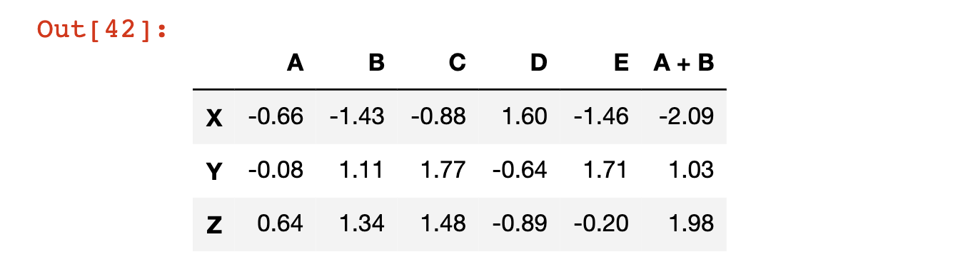
As an example, in the following code block we create a new column called ‘A + B’ which is the sum of columns A and B:

df['A + B'] = df['A'] + df['B']

df 

#The last line prints out the new DataFrame

Here’s the output of that code block:

To remove this column from the pandas DataFrame, we need to use the pd.DataFrame.drop method.

Note that this method defaults to dropping rows, not columns. To switch the method settings to operate on columns, we must pass it in the axis=1 argument.

df.drop('A + B', axis = 1)

It is very important to note that this drop method does not actually modify the DataFrame itself. For evidence of this, print out the df variable again, and notice how it still has the A + B column:

df

The reason that drop (and many other DataFrame methods!) do not modify the data structure by default is to prevent you from accidentally deleting data.

There are two ways to make pandas automatically overwrite the current DataFrame.

The first is by passing in the argument inplace=True, like this:

df.drop('A + B', axis=1, inplace=True)

The second is by using an assignment operator that manually overwrites the existing variable, like this:

df = df.drop('A + B', axis=1)

Both options are valid but I find myself using the second option more frequently because it is easier to remember.

The drop method can also be used to drop rows. For example, we can remove the row Z as follows:

df.drop('Z')

How To Select A Row From A Pandas DataFrame

We have already seen that we can access a specific column of a pandas DataFrame using square brackets. We will now see how to access a specific row of a pandas DataFrame, with the similar goal of generating a pandas Series from the larger data structure.

DataFrame rows can be accessed by their row label using the loc attribute along with square brackets. An example is below.

df.loc['X']

Here is the output of that code:

A   -0.66

B   -1.43

C   -0.88

D    1.60

E   -1.46

Name: X, dtype: float64

DataFrame rows can be accessed by their numerical index using the iloc attribute along with square brackets. An example is below.

df.iloc[0]

As you would expect, this code has the same output as our last example:

A   -0.66

B   -1.43

C   -0.88

D    1.60

E   -1.46

Name: X, dtype: float64

How To Determine The Number Of Rows and Columns in a Pandas DataFrame

There are many cases where you’ll want to know the shape of a pandas DataFrame. By shape, I am referring to the number of columns and rows in the data structure.

Pandas has a built-in attribute called shape that allows us to easily access this:

df.shape

#Returns (3, 5)

Slicing Pandas DataFrames

We have already seen how to select rows, columns, and elements from a pandas DataFrame. In this section, we will explore how to select a subset of a DataFrame. Specifically, let’s select the elements from columns A and B and rows X and Y.

We can actually approach this in a step-by-step fashion. First, let’s select columns A and B:

df[['A', 'B']]

Then, let’s select rows X and Y:

df[['A', 'B']].loc[['X', 'Y']]

And we’re done!

Conditional Selection Using Pandas DataFrame

If you recall from our discussion of NumPy arrays, we were able to select certain elements of the array using conditional operators. For example, if we had a NumPy array called arr and we only wanted the values of the array that were larger than 4, we could use the command arr[arr > 4].

Pandas DataFrames follow a similar syntax. For example, if we wanted to know where our DataFrame has values that were greater than 0.5, we could type df > 0.5 to get the following output:

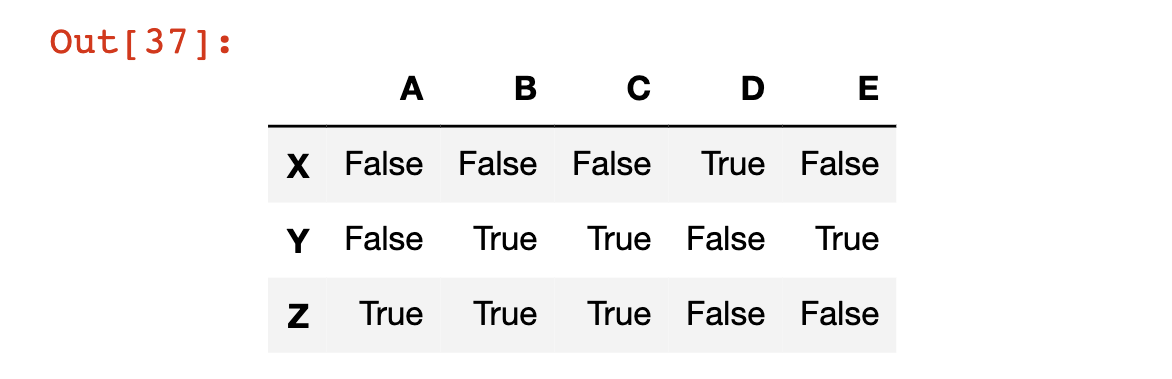
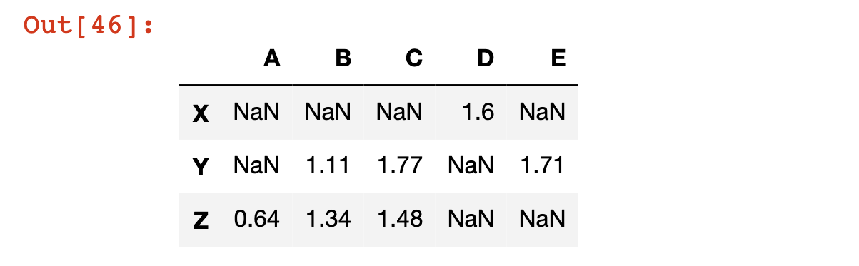
We can also generate a new pandas DataFrame that contains the normal values where the statement is True, and NaN - which stands for Not a Number - values where the statement is false. We do this by passing the statement into the DataFrame using square brackets, like this:

df[df > 0.5]

Here is the output of that code:

You can also use conditional selection to return a subset of the DataFrame where a specific condition is satisfied in a specified column.

To be more specific, let’s say that you wanted the subset of the DataFrame where the value in column C was less than 1. This is only true for row X.

You can get an array of the boolean values associated with this statement like this:

df['C'] < 1

Here’s the output:

X     True

Y    False

Z    False

Name: C, dtype: bool

You can also get the DataFrame’s actual values relative to this conditional selection command by typing df[df['C'] < 1], which outputs just the first row of the DataFrame (since this is the only row where the statement is true for column C:

You can also chain together multiple conditions while using conditional selection. We do this using pandas’ & operator. You cannot use Python’s normal and operator, because in this case we are not comparing two boolean values. Instead, we are comparing two pandas Series that contain boolean values, which is why the & character is used instead.

As an example of multiple conditional selection, you can return the DataFrame subset that satisfies df['C'] > 0 and df['A']> 0 with the following code:

df[(df['C'] > 0) & (df['A']> 0)]

How To Modify The Index of a Pandas DataFrame

There are a number of ways that you can modify the index of a pandas DataFrame.

The most basic is to reset the index to its default numerical values. We do this using the reset_index method:

df.reset_index()

Note that this creates a new column in the DataFrame called index that contains the previous index labels:

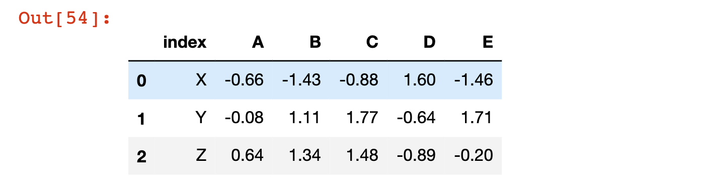
Note that like the other DataFrame operations that we have explored, reset_index does not modify the original DataFrame unless you either (1) force it to using the = assignment operator or (2) specify inplace=True.

You can also set an existing column as the index of the DataFrame using the set_index method. We can set column A as the index of the DataFrame using the following code:

df.set_index('A')

The values of A are now in the index of the DataFrame:

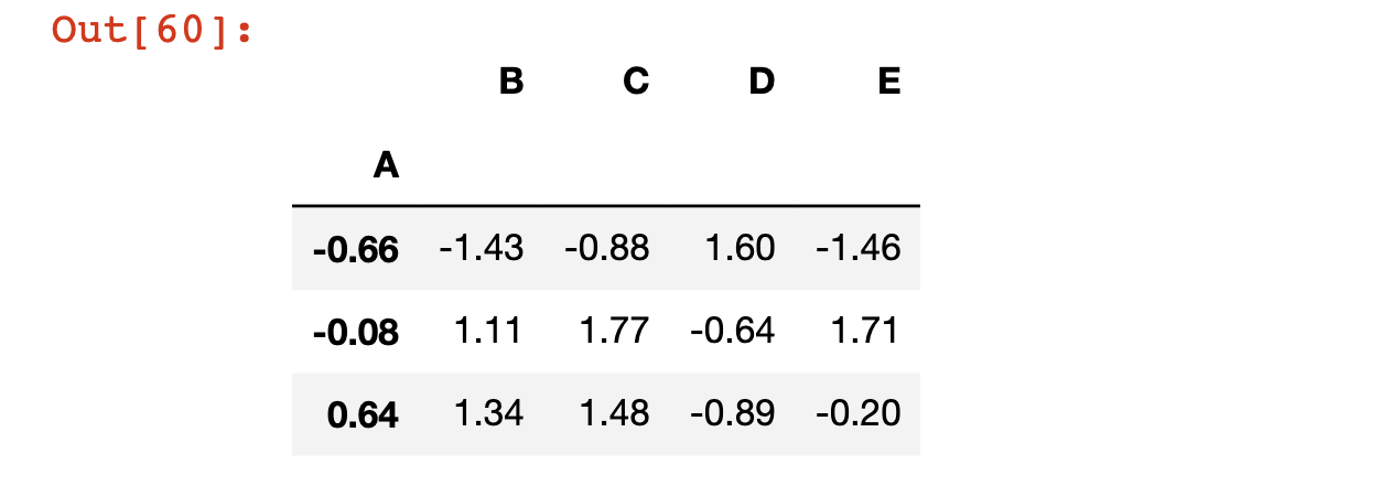
There are three things worth noting here:

• set_index does not modify the original DataFrame unless you either (1) force it to using the = assignment operator or (2) specify inplace=True.
• Unless you run reset_index first, performing a set_index operation with inplace=True or a forced = assignment operator will permanently overwrite your current index values.
• If you want to rename your index to labels that are not currently contained in a column, you can do so by (1) creating a NumPy array with those values, (2) adding those values as a new row of the pandas DataFrame, and (3) running the set_index operation.

How To Rename Columns in a Pandas DataFrame

The last DataFrame operation we’ll discuss is how to rename their columns.

Columns are an attribute of a pandas DataFrame, which means we can call them and modify them using a simple dot operator. For example:

df.columns

#Returns Index(['A', 'B', 'C', 'D', 'E'], dtype='object'

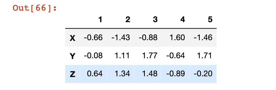
The assignment operator is the best way to modify this attribute:

df.columns = [1, 2, 3, 4, 5]

df

How to Deal With Missing Data in Pandas DataFrames

In an ideal world we will always work with perfect data sets. However, this is never the case in practice. There are many cases when working with quantitative data that you will need to drop or modify missing data. We will explore strategies for handling missing data in Pandas throughout this section.

The DataFrame We’ll Be Using In This section

We will be using the np.nan attribute to generate NaN values throughout this section.

Np.nan

#Returns nan

In this section, we will make use of the following DataFrame:

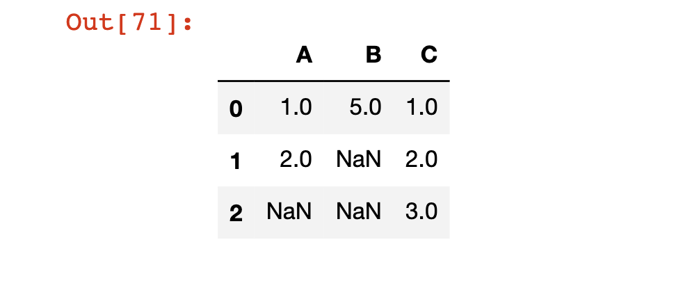
df = pd.DataFrame(np.array([[1, 5, 1],[2, np.nan, 2],[np.nan, np.nan, 3]]))

df.columns = ['A', 'B', 'C']

df

The Pandas dropna Method

Pandas has a built-in method called dropna. When applied against a DataFrame, the dropna method will remove any rows that contain a NaN value.

Let’s apply the dropna method to our df DataFrame as an example:

df.dropna()

Note that like the other DataFrame operations that we have explored, dropna does not modify the original DataFrame unless you either (1) force it to using the = assignment operator or (2) specify inplace=True.

We can also drop any columns that have missing values by passing in the axis=1 argument to the dropna method, like this:

df.dropna(axis=1)

The Pandas fillna Method

In many cases, you will want to replace missing values in a pandas DataFrame instead of dropping it completely. The fillna method is designed for this.

As an example, let’s fill every missing value in our DataFrame with the ?:

df.fillna('?')

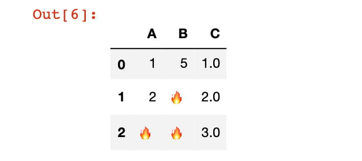
Obviously, there is basically no situation where we would want to replace missing data with an emoji. This was simply an amusing example.

Instead, more commonly we will replace a missing value with either:

• The average value of the entire DataFrame
• The average value of that row of the DataFrame

We will demonstrate both below.

To fill missing values with the average value across the entire DataFrame, use the following code:

df.fillna(df.mean())

To fill the missing values within a particular column with the average value from that column, use the following code (this is for column A):

df['A'].fillna(df['A'].mean())

The Pandas groupby Method

In this section, we will be discussing how to use the pandas groupby feature.

What is the Pandas groupby Feature?

Pandas comes with a built-in groupby feature that allows you to group together rows based off of a column and perform an aggregate function on them. For example, you could calculate the sum of all rows that have a value of 1 in the column ID.

For anyone familiar with the SQL language for querying databases, the pandas groupby method is very similar to a SQL groupby statement.

It is easiest to understand the pandas groupby method using an example. We will be using the following DataFrame:

df = pd.DataFrame([ ['Google', 'Sam', 200],

                    ['Google', 'Charlie', 120],

                    ['Salesforce','Ralph', 125],

                    ['Salesforce','Emily', 250],

                    ['Adobe','Rosalynn', 150],

                    ['Adobe','Chelsea', 500]])

df.columns = ['Organization', 'Salesperson Name', 'Sales']

df

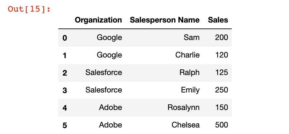
This DataFrame contains sales information for three separate organizations: Google, Salesforce, and Adobe. We will use the groupby method to get summary sales data for each specific organization.

To start, we will need to create a groupby object. This is a data structure that tells Python which column you’d like to group the DataFrame by. In our case, it is the Organization column, so we create a groupby object like this:

df.groupby('Organization')

If you see an output that looks like this, you will know that you have created the object successfully:

<pandas.core.groupby.generic.DataFrameGroupBy object at 0x113f4ecd0>

Once the groupby object has been created, you can call operations on that object to create a DataFrame with summary information on the Organization groups. A few examples are below:

df.groupby('Organization').mean()

#The mean (or average) of the sales column

df.groupby('Organization').sum()

#The sum of the sales column

df.groupby('Organization').std()

#The standard deviation of the sales column

Note that since all of the operations above are numerical, they will automatically ignore the Salesperson Name column, because it only contains strings.

Here are a few other aggregate functions that work well with pandas’ groupby method:

df.groupby('Organization').count()

#Counts the number of observations

df.groupby('Organization').max()

#Returns the maximum value

df.groupby('Organization').min()

#Returns the minimum value

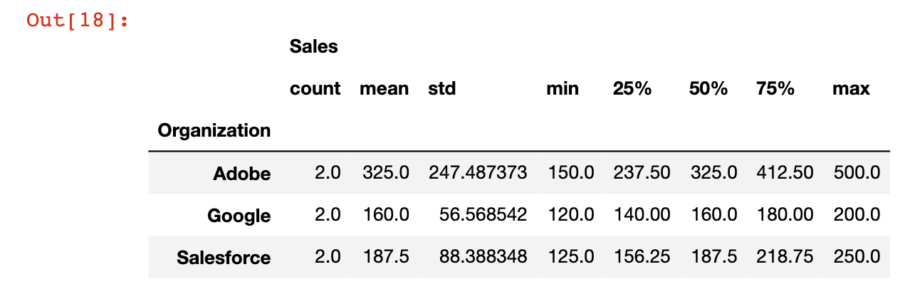
Using groupby With The describe Method

One very useful tool when working with pandas DataFrames is the describe method, which returns useful information for every category that the groupby function is working with.

This is best learned through an example. I’ve combined the groupby and describe methods below:

df.groupby('Organization').describe()

Here is what the output looks like:

The Pandas concat Method

In this section, we will learn how to concatenate pandas DataFrames. This will be a brief section, but it is an important concept nonetheless. Let’s dig in!

The DataFrames We’ll Use In This section

To demonstrate how to merge pandas DataFrames, I will be using the following 3 example DataFrames:

df1 = pd.DataFrame({'A': ['A0', 'A1', 'A2', 'A3'],

                        'B': ['B0', 'B1', 'B2', 'B3'],

                        'C': ['C0', 'C1', 'C2', 'C3'],

                        'D': ['D0', 'D1', 'D2', 'D3']},

                        index=[0, 1, 2, 3])

df2 = pd.DataFrame({'A': ['A4', 'A5', 'A6', 'A7'],

                        'B': ['B4', 'B5', 'B6', 'B7'],

                        'C': ['C4', 'C5', 'C6', 'C7'],

                        'D': ['D4', 'D5', 'D6', 'D7']},

                         index=[4, 5, 6, 7]) 

df3 = pd.DataFrame({'A': ['A8', 'A9', 'A10', 'A11'],

                        'B': ['B8', 'B9', 'B10', 'B11'],

                        'C': ['C8', 'C9', 'C10', 'C11'],

                        'D': ['D8', 'D9', 'D10', 'D11']},

                        index=[8, 9, 10, 11])

How To Concatenate Pandas DataFrames

Anyone who has taken my Introduction to Python course will remember that string concatenation means adding one string to the end of another string. An example of string concatenation is below.

str1 = "Hello "

str2 = "World!"

str1 + str2

#Returns 'Hello World!'

DataFrame concatenation is quite similar. It means adding one DataFrame to the end of another DataFrame.

In order for us to perform string concatenation, we should have two DataFrames with the same columns. An example is below:

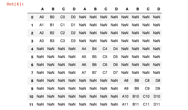
pd.concat([df1, df2, df3])

By default, pandas will concatenate along axis=0, which means that its adding rows, not columns.

If you want to add rows, simply pass in axis=0 as a new variable into the concat function.

pd.concat([df1,df2,df3],axis=1)

In our case, this creates a very ugly DataFrame with many missing values:

The Pandas merge Method

In this section, we’ll learn how to merge pandas DataFrames.

The DataFrames We Will Be Using In This section

In this section, we will be using the following two pandas DataFrames:

import pandas as pd

leftDataFrame = pd.DataFrame({'key': ['K0', 'K1', 'K2', 'K3'],

                     'A': ['A0', 'A1', 'A2', 'A3'],

                     'B': ['B0', 'B1', 'B2', 'B3']})

   

rightDataFrame = pd.DataFrame({'key': ['K0', 'K1', 'K2', 'K3'],

                          'C': ['C0', 'C1', 'C2', 'C3'],

                          'D': ['D0', 'D1', 'D2', 'D3']})    

The columns A, B, C, and D have real data in them, while the column key has a key that is common among both DataFrames. To merge two DataFrames means to connect them along one column that they both have in common.

How To Merge Pandas DataFrames

You can merge two pandas DataFrames along a common column using the merge columns. For anyone that is familiar with the SQL programming language, this is very similar to performing an inner join in SQL.

Do not worry if you are unfamiliar with SQL, because merge syntax is actually very straightforward. It looks like this:

pd.merge(leftDataFrame, rightDataFrame, how='inner', on='key')

Let’s break down the four arguments we passed into the merge method:

1. leftDataFrame: This is the DataFrame that we’d like to merge on the left.
2. rightDataFrame: This is the DataFrame that we’d like to merge on the right.
3. how=inner: This is the type of merge that the operation is performing. There are multiple types of merges, but we will only be covering inner merges in this course.
4. on='key': This is the column that you’d like to perform the merge on. Since key was the only column in common between the two DataFrames, it was the only option that we could use to perform the merge.

The Pandas join Method

In this section, you will learn how to join pandas DataFrames.

The DataFrames We Will Be Using In This Section

We will be using the following two DataFrames in this section:

leftDataFrame = pd.DataFrame({  'A': ['A0', 'A1', 'A2', 'A3'],

                                'B': ['B0', 'B1', 'B2', 'B3']},

                                index =['K0', 'K1', 'K2', 'K3'])

   

rightDataFrame = pd.DataFrame({ 'C': ['C0', 'C1', 'C2', 'C3'],

                                'D': ['D0', 'D1', 'D2', 'D3']},

                                index = ['K0', 'K1', 'K2', 'K3'])  

If these look familiar, it’s because they are! These are the nearly the same DataFrames as we used when learning how to merge pandas DataFrames. A key difference is that instead of the key column being its own column, it is now the index of the DataFrame. You can think of these DataFrames as being those from the last section after executing .set_index(key).

How To Join Pandas DataFrames

Joining pandas DataFrames is very similar to merging pandas DataFrames except that the keys on which you’d like to combine are in the index instead of contained within a column.

To join these two DataFrames, we can use the following code:

leftDataFrame.join(rightDataFrame)

Other Common Operations in Pandas

This section will explore common operations in the pandas Python library. The purpose of this section is to explore important pandas operations that have not fit into any of the sections we’ve discussed so far.

The DataFrame We Will Use In This section

I will be using the following DataFrame in this section:

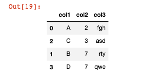
df = pd.DataFrame({'col1':['A','B','C','D'],

                   'col2':[2,7,3,7],

                   'col3':['fgh','rty','asd','qwe']})

How To Find Unique Values in a Pandas Series

Pandas has an excellent method called unique that can be used to find unique values within a pandas Series. Note that this method only works on Series and not on DataFrames. If you try to apply this method to a DataFrame, you will encounter an error:

df.unique()

#Returns AttributeError: 'DataFrame' object has no attribute 'unique'

However, since the columns of a pandas DataFrame are each a Series, we can apply the unique method to a specific column, like this:

df['col2'].unique()

#Returns array([2, 7, 3])

Pandas also has a separate nunique method that counts the number of unique values in a Series and returns that value as an integer. For example:

df['col2'].nunique()

#Returns 3

Interestingly, the nunique method is exactly the same as len(unique()) but it is a common enough operation that the pandas community decided to create a specific method for this use case.

How To Count The Occurence of Each Value In A Pandas Series

Pandas has a function called counts_value that allows you to easily count the number of time each observation occurs. An example is below:

df['col2'].value_counts()

"""

Returns:

7    2

2    1

3    1

Name: col2, dtype: int64

"""

How To Use The Pandas apply Method

The apply method is one of the most powerful methods available in the pandas library. It allows you to apply a custom function to every element of a pandas Series.

As an example, imagine that we had the following function exponentify that takes in an integer and raises it to the power of itself:

def exponentify(x):

    return x**x

The apply method allows you to easily apply the exponentify function to each element of the Series:

df['col2'].apply(exponentify)

"""

Returns:

0         4

1    823543

2        27

3    823543

Name: col2, dtype: int64

"""

The apply method can also be used with built-in functions like len (although it is definitely more powerful when used with custom functions). An example of the len function being used in conjunction with apply is below:

df['col3'].apply(len)

"""

Returns

0    3

1    3

2    3

3    3

Name: col3, dtype: int64

"""

How To Sort A Pandas DataFrame

You can filter a pandas DataFrame by the values of a particular column using the sort_values method. As an example, if you wanted to sort by col2 in our DataFrame df, you would run the following command:

df.sort_values('col2')

The output of this command is below:

There are two things to note from this output:

1. As you can see, each row preserves its index, which means the index is now out of order.
2. As with the other DataFrame methods, this does not actually modify the original DataFrame unless you force it to using the = assignment operator or by passing in inplace = True.

Local Data Input and Output (I/O) in Pandas

In this section, we will begin exploring data input and output with the pandas Python library.

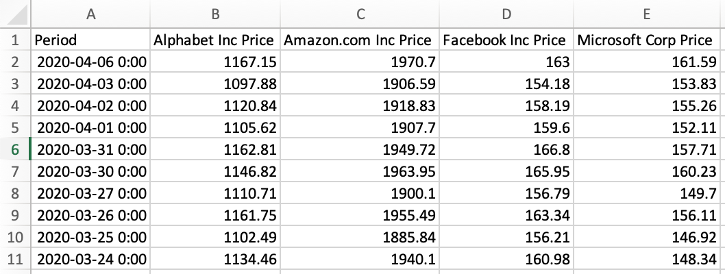
The File We Will Be Working With In This section

We will be working with different files containing stock prices for Facebook (FB), Amazon (AMZN), Google (GOOG), and Microsoft (MSFT) in this section. To download these files, download the entire GitHub repository for this course here. The files used in this section can be found in the stock_prices folder of the repository.

You’ll want to save these files in the same directory as your Jupyter Notebook for this section. The easiest way to do this is to download the GitHub repository, and then open your Jupyter Notebook in the stock_prices folder of the repository.

How To Import .csv Files Using Pandas

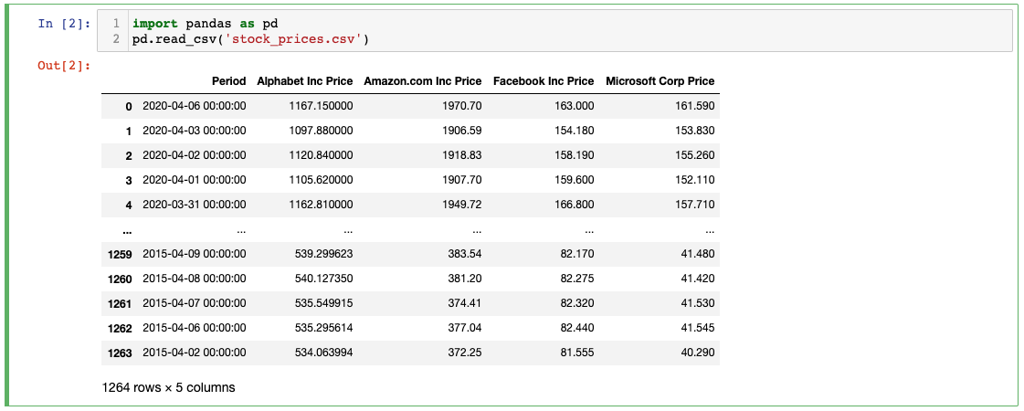
We can import .csv files into a pandas DataFrame using the read_csv method, like this:

import pandas as pd

pd.read_csv('stock_prices.csv')

As you’ll see, this creates (and displays) a new pandas DataFrame containing the data from the .csv file.

You can also assign this new DataFrame to a variable to be referenced later using the normal = assignment operator:

new_data_frame = pd.read_csv('stock_prices.csv')

There are a number of read methods included with the pandas programming library. If you are trying to import data from an external document, then it is likely that pandas has a built-in method for this.

A few examples of different read methods are below:

pd.read_json()

pd.read_html()

pd.read_excel()

We will explore some of these methods later in this section.

If we wanted to import a .csv file that was not directly in our working directory, we need to modify the syntax of the read_csv method slightly.

If the file is in a folder deeper than what you’re working in now, you need to specify the full path of the file in the read_csv method argument. As an example, if the stock_prices.csv file was contained in a folder called new_folder, then we could import it like this:

new_data_frame = pd.read_csv('./new_folder/stock_prices.csv')

For those unfamiliar with working with directory notation, the . at the start of the filepath indicates the current directory. Similarly, a .. indicates one directory above the current directory, and a ...indicates two directories above the current directory.

This syntax (using periods) is exactly how we reference (and import) files that are above our current working directory. As an example, open a Jupyter Notebook inside the new_folder folder, and place stock_prices.csv in the parent folder. With this file layout, you could import the stock_prices.csv file using the following command:

new_data_frame = pd.read_csv('../stock_prices.csv')

Note that this directory syntax is the same for all types of file imports, so we will not be revisiting how to import files from different directories when we explore different import methods later in this course.

How To Export .csv Files Using Pandas

To demonstrate how to save a new .csv file, let’s first create a new DataFrame. Specifically, let’s fill a DataFrame with 3 columns and 50 rows with random data using the np.random.randn method:

import pandas as pd

import numpy as np

df = pd.DataFrame(np.random.randn(50,3))

Now that we have a DataFrame, we can save it using the to_csv method. This method takes in the name of the new file as its argument.

df.to_csv('my_new_csv.csv')

You will notice that if you run the code above, the new .csv file will begin with an unlabeled column that contains the index of the DataFrame. An example is below (after opening the .csv in Microsoft Excel):

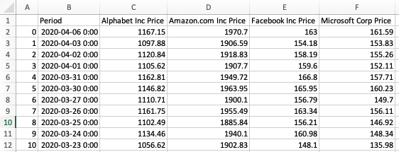
In many cases, this is undesirable. To remove the blank index column, pass in index=False as a second argument to the to_csv method, like this:

new_data_frame.to_csv('my_new_csv.csv', index = False)

The new .csv file does not have the unlabelled index column:

The read_csv and to_csv methods make it very easy to import and export data from .csv files using pandas. We will see later in this section that for every read method that allows us to import data, there is usually a corresponding to function that allows us to save that data!

How To Import .json Files Using Pandas

If you are not experienced in working with large datasets, then you may not be familiar with the JSON file type.

JSON stands for JavaScript Object Notation. JSON files are very similar to Python Dictionaries.

JSON files are one of the most commonly-used data types among software developers because they can be manipulated using basically every programming language.

Pandas has a method called read_json that makes it very easy to import JSON files as a pandas DataFrame. An example is below.

json_data_frame = pd.read_json('stock_prices.json')

We’ll learn how to export JSON files next.

How To Export .json Files Using Pandas

As I mentioned earlier, there is generally a to method for every read method. This means that we can save a DataFrame to a JSON file using the to_json method.

As an example, let’s take the randomly-generated DataFrame df from earlier in this section and save it as a JSON file in our local directory:

df.to_json('my_new_json.json')

We’ll learn how to work with Excel files - which have the file extension .xlsx - next.

How To Import .xlsx Files Using Pandas

Pandas’ read_excel method makes it very easy to import data from an Excel document into a pandas DataFrame:

new_data_frame = pd.read_excel('stock_prices.xlsx')

Unlike the read_csv and read_json methods that we explored earlier in this section, the read_excel method can accept a second argument. The reason why read_excel accepts multiple arguments is that Excel spreadsheets can contain multiple sheets. The second argument specifies which sheet you are trying to import and is called sheet_name.

As an example, if our stock_prices had a second sheet called Sheet2, you would import that sheet to a pandas DataFrame like this:

new_data_frame.to_excel('stock_prices.xlsx', sheet_name='Sheet2')

If you do not specify any value for sheet_name, then read_excel will import the first sheet of the Excel spreadsheet by default.

While importing Excel documents, it is very important to note that pandas only imports data. It cannot import other Excel capabilities like formatting, formulas, or macros. Trying to import data from an Excel document that has these features may cause pandas to crash.

How To Export .xlsx Files Using Pandas

Exporting Excel files is very similar to importing Excel files, except we use to_excel instead of read_excel. An example is below using our randomly-generated df DataFrame:

df.to_excel('my_new_excel_file.xlsx')

Like read_excel, to_excel accepts a second argument called sheet_name that allows you to specify the name of the sheet that you’re saving. For example, we could have named the sheet of the new .xlsx file My New Sheet! by passing it into the to_excel method like this:

df.to_excel('my_new_excel_file.xlsx', sheet_name='My New Sheet!')

If you do not specify a value for sheet_name, then the sheet will be named Sheet1 by default (just like when you create a new Excel document using the actual application).

Remote Data Input and Output (I/O) in Pandas

In the last section of this course, we learned how to import data from .csv, .json, and .xlsx files that were saved on our local computer. We will follow up by showing you how you can import files without actually saving them to your local machine first. This is called remote importing.

What Is Remote Importing and Why Is It Useful?

Remote importing means bringing a file into your Python script without having that file saved on your computer.

On the surface, it may not seem clear why we might want to engage in remote importing. However, it can be very useful.

The reason why remote importing is useful is because, by definition, it means the Python script will continue to function even if the file being imported is not saved on your computer. This means I can send my code to colleagues or friends and it will still function properly.

Throughout the rest of this section, I will demonstrate how to perform remote imports in pandas for .csv, .json, and .xlsx files.

How To Import Remote .csv Files

First, navigate to this course’s GitHub Repository. Open up the stock_prices folder. Click on the file stock_prices.csv and then click the button for the Raw file, as shown below.

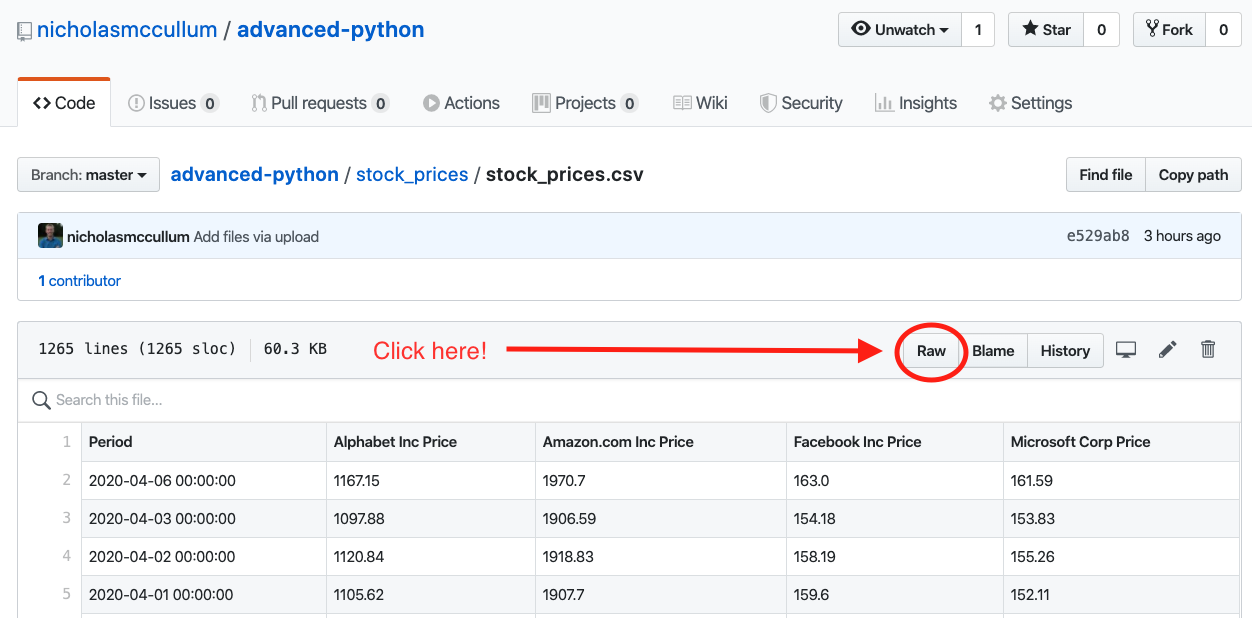
This will take you to a new page that has the data from the .csv file contained within stock_prices.csv.

To import this remote file into your into your Python script, you must first copy its URL to your clipboard. You can do this by either (1) highlighting the entire URL, right-clicking the selected text, and clicking copy, or (2) highlighting the entire URL and typing CTRL+C on your keyboard.

The URL will look like this:

[https://raw.githubusercontent.com/nicholasmccullum/advanced-python/master/stock_prices/stock_prices.csv](https://raw.githubusercontent.com/nicholasmccullum/advanced-python/master/stock_prices/stock_prices.csv)

You can pass this URL into the read_csv method to import the dataset into a pandas DataFrame without saving the dataset to your computer first:

pd.read_csv('https://raw.githubusercontent.com/nicholasmccullum/advanced-python/master/stock_prices/stock_prices.csv')

How To Import Remote .json Files

We can import remote .json files in a similar fashion to .csv files.

First, grab the raw URL from GitHub. It will look like this:

https://raw.githubusercontent.com/nicholasmccullum/advanced-python/master/stock_prices/stock_prices.json

Next, pass this URL into the read_json method like this:

pd.read_json('https://raw.githubusercontent.com/nicholasmccullum/advanced-python/master/stock_prices/stock_prices.json')

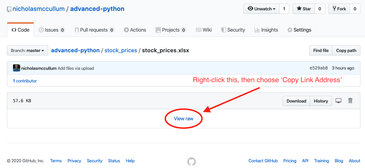
How To Import Remote .xlsx Files

We can import remote .xlsx files in a similar fashion to .csv and .json files. Note that you will need to click in a slightly different place on the GitHub interface. Specifically, you’ll need to right-click ‘View Raw’ and select ‘Copy Link Address,’ as shown below.

The raw URL will look like this:

https://github.com/nicholasmccullum/advanced-python/blob/master/stock_prices/stock_prices.xlsx?raw=true

Then, pass this URL into the read_excel method, like this:

pd.read_excel('https://github.com/nicholasmccullum/advanced-python/blob/master/stock_prices/stock_prices.xlsx?raw=true')

The Downsides to Remote Importing

Remote importing means that you do not need to first save the file being imported onto your local computer, which is an unquestionable benefit.

However, remote importing also has two downsides:

1. You must have an Internet connection to perform remote imports
2. Pinging the URL to retrieve the dataset is fairly time-consuming, which means that performing remote imports will slow the speed of your Python code

Final Thoughts & Special Offer

Thanks for reading this article on Pandas, which is one of my favorite Python packages and a must-know library for every Python developer.

This tutorial is an excerpt from my course Python For Finance and Data Science. If you're interested in learning more core Python skills, the course is 50% off for the first 50 freeCodeCamp readers that sign up - click here to get your discounted course now!