

Machine learning need not be mysterious. A lot of the basics come wrapped up in high-level software packages such as scikit-learn, but you can actually do a lot without ever having to leave the database.
PostgreSQL lets you build queries which run a variety of machine learning algorithms against your data.
Here, I demonstrate four popular machine learning algorithms written entirely in SQL.
I'll present these queries in a way that allows for ease of exposition, but they're not intended for use in a production setting.
Regardless, working through them is a great way to test your knowledge of both machine learning and SQL, as well as problem solving - essential skills for any data scientist.
Linear regression
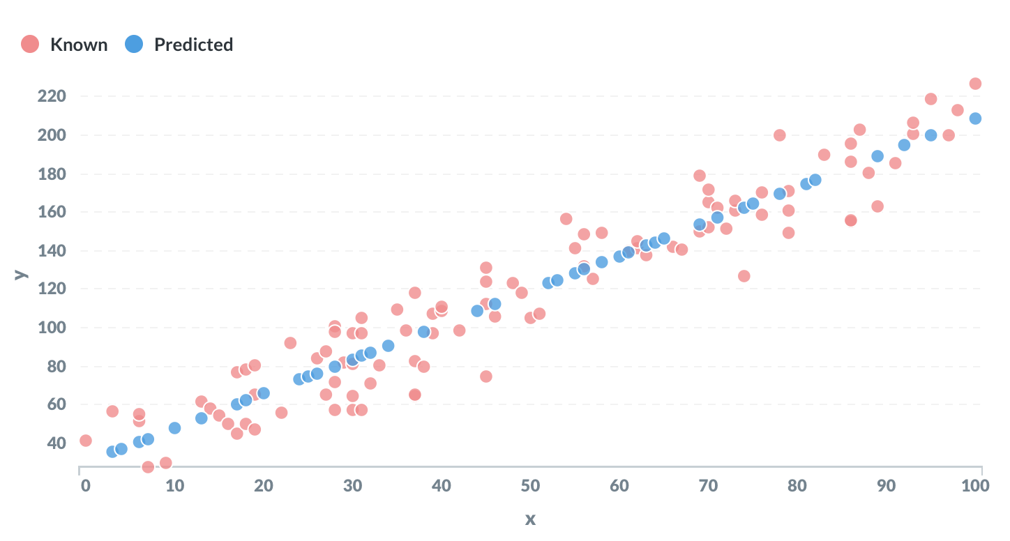
Linear regression is perhaps the most elementary example of machine learning. The objective is to “learn” the parameters m and c of a linear equation of the form y = mx + c from a set of training data.
This is a great example of the statistical functions that come inbuilt with PostgreSQL.
The input data is in a table with two columns:
x | y
Some values of y are set to NULL. The goal is to predict these missing values.
WITH regression AS
  (SELECT
      regr_slope(y, x) AS gradient,
      regr_intercept(y, x) AS intercept
   FROM
      linear_regression
   WHERE
      y IS NOT NULL
   )

SELECT
   x,
   (x * gradient) + intercept AS prediction
FROM
   linear_regression
CROSS JOIN
   regression
WHERE
   y IS NULL ;
The regr_slope() and regr_intercept() functions are used to estimate the gradient and intercept terms respectively. These correspond to the parameters m and c in the equation.
The output will be all the unknown points, with a predicted value for y based on the value of x.
K-Nearest Neighbours
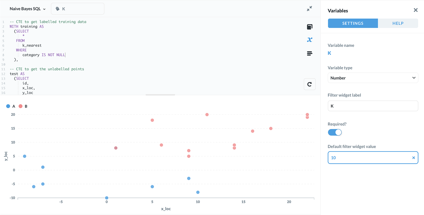
K-nearest neighbours is a classic example of a supervised classification algorithm. The premise is quite straightforward. Each data point is represented as a point in space, labeled as one of any number of categories or classes.
To classify an unlabelled data point, simply look at the labels of the points closest to it. Whichever label appears most frequently is used as an estimate.
The number of neighbouring points considered is determined by a parameter K.
Here, the input data is a table with the following columns:
id | x_loc | y_loc | category
Some of the values in the category column are NULL. The goal is to classify these using the K-nearest neighbours algorithm.
-- CTE to get labelled training data
WITH training AS
  (SELECT
      id,
      POINT(x_loc, y_loc) as xy,
      category
  FROM
      k_nearest
  WHERE
      category IS NOT NULL
  ),

-- CTE to get the unlabelled points
test AS
  (SELECT
      id,
      POINT(x_loc, y_loc) as xy,
      category
  FROM
      k_nearest
  WHERE
      category IS NULL
  ),

-- calculate distances between unlabelled & labelled points
distances AS
  (SELECT
      test.id,
      training.category,
      test.xy <-> training.xy AS dist,
      ROW_NUMBER() OVER (
         PARTITION BY test.id
         ORDER BY test.xy <-> training.xy
         ) AS row_no
  FROM
      test
  CROSS JOIN training
  ORDER BY 1, 4 ASC
  ),

-- count the 'votes' per label for each unlabelled point
votes AS
  (SELECT
      id,
      category,
      count(*) AS votes
  FROM distances
  WHERE row_no <= {{K}}
  GROUP BY 1,2
  ORDER BY 1)

-- query for the label with the most votes
SELECT
  v.id,
  v.category
FROM
  votes v
JOIN
  (SELECT
      id,
      max(votes) AS max_votes
  FROM
      votes
  GROUP BY 1
  ) mv
ON v.id = mv.id
AND v.votes = mv.max_votes
ORDER BY 1 ASC ;
In the query above, the parameter K is written as a variable {{K}}. If you use a tool such as Metabase, you can input different values of K and see what effect they have.
The query makes use of PostgreSQL’s POINT() data type and distance operator to calculate the distances between the data.
The output will be each of the unlabelled points, along with the estimated class.
Naive Bayes classification
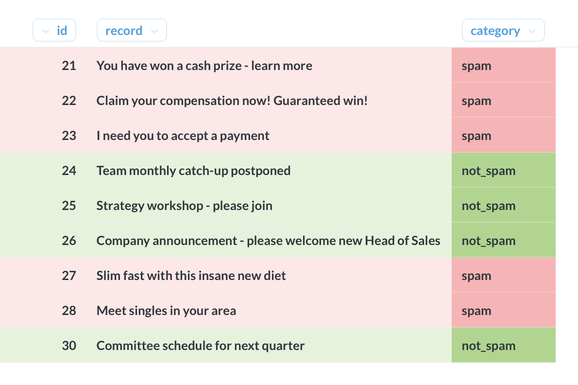
Naive Bayes classification is a technique used for classification tasks as varied as spam detection through to document classification and sentiment analysis.
It works by using Bayes rule to relate the “probability of the class, given the data” to the “probability of the data, given the class”. The latter can be readily estimated from a set of labelled training data.
The query below takes as input a table with the following columns:
id | record | category
Here, record is a piece of text (e.g, email subject line) and category is one of several possible classes (e.g, spam or not spam).
For some rows, category is set to NULL. The goal is to estimate the missing categories using Naive Bayes classification.
-- CTE to create one row per word
WITH staging AS
  (SELECT
      REGEXP_SPLIT_TO_TABLE(
         LOWER(record), '[^a-z]+') AS word,
      category
   FROM
      naive_bayes
   WHERE
      category IS NOT NULL
  ),

-- testing data
test AS
  (SELECT
      id,
      record
   FROM
      naive_bayes
   WHERE
      category is NULL
  ),

-- one row per word + category
cartesian AS
  (SELECT
      *
   FROM
     (SELECT
         DISTINCT word
      FROM
         staging) w
      CROSS JOIN
     (SELECT
         DISTINCT category
      FROM
         staging) c
      WHERE
         length(word) > 0
   ),

-- CTE of smoothed frequencies of each word by category
frequencies AS
  (SELECT
      c.word,
      c.category,
      -- numerator plus one
      (SELECT
          count(*)+1
       FROM
          staging s
       WHERE
          s.word = c.word
       AND
          s.category = c.category) /
      -- denominator plus two
      (SELECT
          count(*)+2
       FROM
          staging s1
       WHERE
          s1.category = c.category) ::DECIMAL AS freq
   FROM
      cartesian c
   ),

-- for each row in testing, get the probabilities
probabilities AS
  (SELECT
      t.id,
      f.category,
      SUM(LN(f.freq)) AS probability
   FROM
     (SELECT
         id,
         REGEXP_SPLIT_TO_TABLE(
            LOWER(record), '[^a-z]+') AS word
      FROM
         test) t
   JOIN
     (SELECT
         word,
         category,
         freq
      FROM
         frequencies) f
   ON t.word = f.word
   GROUP BY 1, 2
  )

-- keep only the highest estimate
SELECT
   record,
   probabilities.category
FROM
   probabilities
JOIN
  (SELECT
      id,
      max(probability) AS max_probability
   FROM
      probabilities
   GROUP BY 1) p
ON probabilities.id = p.id
AND probabilities.probability = p.max_probability
JOIN
   test
ON probabilities.id = test.id
ORDER BY 1 ;
The output is each of the unclassified records, with a predicted category assigned.
The query above makes a few simplifications. For one, the only preprocessing of the text data is a simple regular expression to keep the letters A-Z, and the use of the LOWER() function to coerce everything to lower case.
It also assumes a uniform prior probability for each of the classes (in other words, the assumption is before looking at the data, spam and non-spam emails are equally likely).
K-means clustering
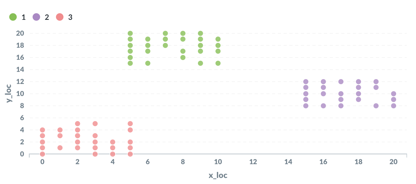
K-means clustering is a well-known classification algorithm. It is an unsupervised algorithm, meaning it does not require any labelled training data.
K-means clustering works by representing each data point as a point in space. Each point is initially assigned at random to one of K clusters (where K is a parameter chosen in advance).
Next, the average location of the points is calculated for each cluster.
Then, each point is reassigned to the cluster with the nearest average location.
These two steps are repeated over and over until the points are no longer reassigned between steps.
The input data is a table with the following columns:
id | x_loc | y_loc
The output is the full set of points, each assigned to one of K clusters.
This one was tough to implement. The solution below is heavily based on a generalisation of this purchase data example created by Jim Nasby under a BSD 2-clause license (which applies below).
WITH points AS
   (SELECT
       id,
       POINT(x_loc, y_loc) AS xy
    FROM
       k_means_clustering
    ),

initial AS
   (SELECT
       RANK() OVER (
          ORDER BY random()
       ) AS cluster,
       xy
    FROM points
    LIMIT {{K}}
    ),

iteration AS
   (WITH RECURSIVE kmeans(iter, id, cluster, avg_point) AS (
       SELECT
          1,
          NULL::INTEGER,
          *
        FROM
           initial
        UNION ALL
        SELECT
           iter + 1,
           id,
           cluster,
           midpoint
        FROM (
           SELECT DISTINCT ON(iter, id)
              *
           FROM (
              SELECT
                 iter,
                 cluster,
                 p.id,
                 p.xy <-> k.avg_point AS distance,
                 @@ LSEG(p.xy, k.avg_point) AS midpoint,
                 p.xy,
                 k.avg_point
               FROM points p
               CROSS JOIN kmeans k
               ) d
            ORDER BY 1, 3, 4
            ) r
       WHERE iter < {{max_iter}}
   )
   SELECT
      *
   FROM
      kmeans
   )

SELECT
   k.*,
   cluster
FROM
   iteration i
JOIN
   k_means_clustering k
USING(id)
WHERE
   iter = {{max_iter}}
ORDER BY 4,1 ASC ;
This query makes use of a couple of neat features.
For one, it makes use of PostgreSQL’s geometric data types and operators to model the data in terms of points and line segments.
It also uses a recursive query to iteratively recalculate the centres of each cluster up to a maximum number of iterations.
This implementation uses a predefined number of iterations before terminating, rather than stopping once the points stop being reassigned between iterations.
If you use a tool such as Metabase, you can set the parameters K and maximum number of iterations dynamically using the variables {{K}} and {{max_iter}}.
Summary
SQL is a powerful language capable of much more than simply storing and loading data in databases.
It is a declarative language, so you have to describe the result you are looking for (as opposed to an imperative language, where you give the computer instructions step-by-step).
This requires thinking about machine learning problems in a different way, but it is still possible to achieve some interesting results.
All of the sample data and queries used in this article can be found here.
If you enjoyed this article, you may also be interested in Learn these quick tricks in PostgreSQL and How to use fuzzy string matching with PostgreSQL.
You can follow more of my writing at gleeson.substack.com