

In Artificial Intelligence, Machine Learning is the foundation of most revolutionary AI applications. From language processing to image recognition, Machine Learning is everywhere.
Machine Learning relies on algorithms, statistical models, and neural networks. And Deep Learning is the subfield of Machine Learning focused only on neural networks.
A key piece of any neural network are activation functions. But understanding exactly why they are essential to any neural network system is a common question, and it can be a difficult one to answer.
This tutorial focuses on explaining, in a simple manner with analogies, why exactly activation functions are necessary.
By understanding this, you will understand the process of how AI models think.
Before that, we will explore neural networks in AI. We will also explore the most commonly used activation functions.
We're also going to analyze every line of a very simple PyTorch code example of a neural network.
In this article, we will explore:
- Artificial Intelligence and the Rise of Deep Learning
- Understanding Activation Functions: Simplifying Neural Network Mechanics
- Simple Analogy: The Necessity of Activation Functions
- What Happens Without Activation Functions?
- PyTorch Activation Function Code Example
- Conclusion: The Unsung Heroes of AI Neural Networks
This article won't cover dropout or other regularization techniques, hyperparameter optimization, complex architectures like CNNs, or detailed differences in gradient descent variants.
I just want to showcase why activation functions are needed and what happens when they are not applied to neural networks.
If you don't know much about deep learning, I personally recommend this Deep Learning crash course on freeCodeCamp's YouTube channel:
Artificial Intelligence and the Rise of Deep Learning
What is Deep Learning in Artificial Intelligence?
Deep learning is a subfield of artificial intelligence. It uses neural networks to process complex patterns, just like the strategies a sports team uses to win a match.
The bigger the neural network, the more capable it is of doing awesome things – like ChatGPT, for example, which uses natural language processing to answer questions and interact with users.
To truly understand the basics of neural networks – what every single AI model has in common that enables it to work – we need to understand activation layers.
Deep Learning = Training Neural Networks
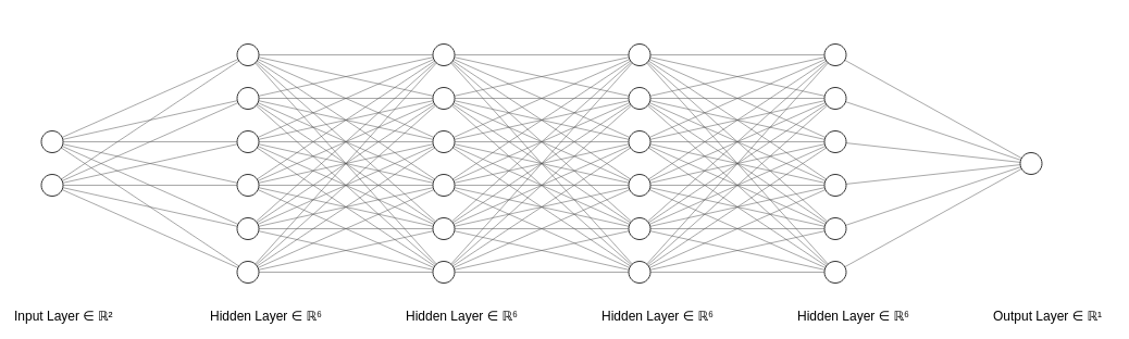
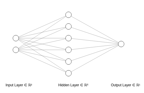
 Simple neural network
At the core of deep learning is the training of neural networks.
That means basically using data to get the right values of the weights to be able to predict what we want.
Neural networks are made of neurons organized in layers. Each layer extracts unique features from the data.
This layered structure allows deep learning models to analyze and interpret complex data.
Understanding Activation Functions: Simplifying Neural Network Mechanics
 Leaky reLU activation function
Activation functions help neural networks handle complex data. They change the neuron value based on the data they receive.
It is almost like a filter every neuron has before sending its value to the next neuron.
Essentially, activation functions control the information flow of neural networks – they decide which data is relevant and which is not.
This helps prevent the vanishing gradients to ensure the network learns properly.
The vanishing gradients problem happens when the neural network's learning signals are too weak to make the weight values change. This makes learning from data very difficult.
Simple Analogy: Why Activation Functions are Necessary
In a soccer game, players decide whether to pass, dribble, or shoot the ball.
These decisions are based on the current game situation, just as neurons in a neural network process data.
In this case, activation functions act like this in the decision-making process.
Without them, neurons would pass data without any selective analysis – like players mindlessly kicking the ball regardless of the game context.
In this way, activation functions introduce complexity into a neural network, allowing it to learn complex patterns.
What Happens Without Activation Functions?
To understand what would happen without activation functions, let's first think about what happens if players mindlessly kick the ball in a soccer match.
They'd likely lose the match because there would be no decision-making processes as a team. That ball still goes somewhere – but most of the time it will not go where it's intended.
This is similar to what happens in a neural network without activation functions: the neural network doesn't make good predictions because the neurons were just passing data to each other randomly.
We still get a prediction. Just not what we wanted, or what's helpful.
This dramatically limits the capability – of both the soccer team and the neural network.
Intuitive Explanation of Activation Functions
Let's now look at an example so you can understand this intuitively.
 reLU activation function
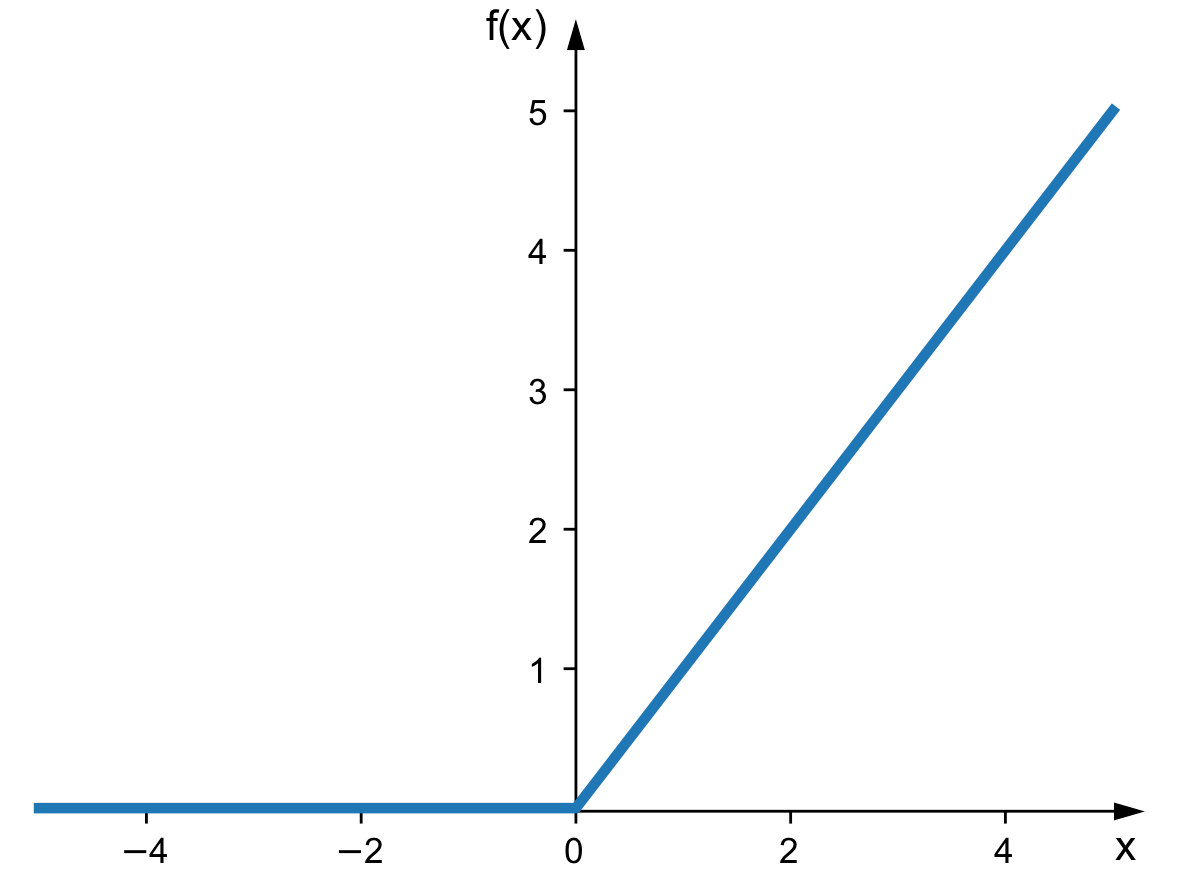
Let's start with the most widely used activation function in deep learning (it's also one of the simpler ones).
This is an ReLU activation function. It basically acts as a filter before a neuron sends a value to its next neuron.
This filter is essentially two conditions:
- If the value of the weight is negative, it becomes 0
- If the value of the weight is positive, it does not change anything
With this, we are adding a decision-making process to each neuron. It decides which data to send and which not to send.
Now let's look at some examples of other activation functions.
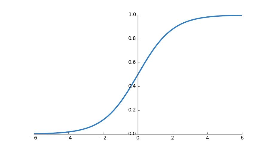
Sigmoid Activation Functions
This activation function converts the input value between 0 and 1. Sigmoids are widely used in binary classification problems in the last neuron.
 Sigmoid activation function
There is a problem with sigmoid activation functions, though. Take the output values from a given linear transformation:
- 0.00000003
- 0.99999992
- 0.00000247
- 0.99993320
There are some questions about these values we can ask:
- Are values like 0.00000003 and 0.000002 really important? Can't they be just 0 so that we have fewer things to run on the computer? Remember, in many of today's models, we have millions of weights in them. Can't millions of 0.00000003 and 0.000002 be 0?
- And if it is a positive value, how will it distinguish a big value from a very big value? For example, in 0.99993320 and 0.99999992, where are the input values like 7 and 13 or 7 and 55? 0.99993320 and 0.99999992 do not accurately describe their input values.
How can we distinguish the subtle differences in outputs so that accuracy is maintained?
This is what the ReLU activation functions solved: setting negative numbers to zero while keeping positive ones boosts neural network computational efficiency.
Tanh (Hyperbolic Tangent) Activation Functions
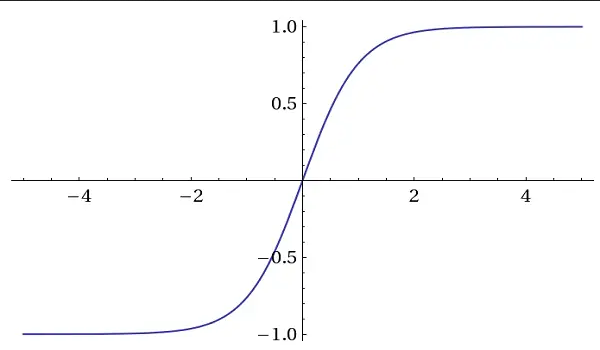 tanh activation function
These activation functions output values between -1 and 1, similar to Sigmoid.
They're often used in recurrent neural networks (RNNs) and long short-term memory networks (LSTMs).
Tanh is also used because it is zero-centered. This means that the mean of the output values is around zero. This property helps when dealing with the vanishing gradient problem.
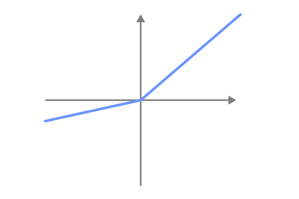
Leaky reLU
 Leaky reLU activation function
Instead of ignoring the negative values, Leaky ReLU activation functions are going to have a small negative value.
This way, negative values are also used when training neural networks.
With the ReLU activation function, neurons with negative values are inactive and do not contribute to the learning process.
With the Leaky ReLU activation function, neurons with negative values are active and contribute to the learning process.
This decision-making process is implemented by activations function. Without it, it would simply send the data to the next neuron (just like a player mindlessly kicking the ball).
Mathematical Explanation of Activation Functions
Neurons do two things:
- They use linear transformations with the previous neurons weights values
- They use activation functions to filter certain values to selectively pass on values.
Without activation functions, the neural network just does one thing: Linear transformations.
If it only does linear transformations, it is a linear system.
If it is a linear system, in very simple terms without being too technical, the superposition theorem tells us that any mixture of two or more linear transformations can be simplified into one single transformation.
Essentially, it means that, without activation functions, this complex neural network:
 Long neural network without activation functions
Is the same as this simple one:
 Short neural network without activation functions
This is because each layer in its matrix form is a product of linear transformations of previous layers.
And according to the theorem, since any mixture of two or more linear transformations can be simplified in one single transformation, then any mixture of hidden layers (that is, layers between the inputs and outputs of neurons) in a neural network can be simplified into only one layer.
What does this all mean?
It means that it can only model data linearly. But in real life with real data, every system is non-linear. So we need activation functions.
We introduce non-linearity into a neural network so that it learns non-linear patterns.
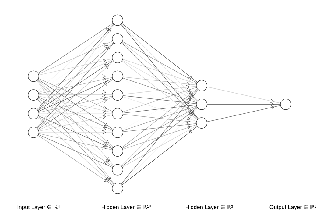
PyTorch Activation Function Code Example
In this section, we are going to train the neural network below:
 Simple feed forward neural network
This is a simple neural network AI model with four layers:
- Input layer with 10 neurons
- Two hidden layers with 18 neurons
- One hidden layer with 18 neurons
- One output layer with 1 neuron
In the code, we can choose any of the four activation functions mentioned in this tutorial.
Here it is the full code – we'll discuss in detail below:
import torch
import torch.nn as nn
import torch.optim as optim

#Choose which activation function to use in code
defined_activation_function = 'relu'

activation_functions = {
    'relu': nn.ReLU(),
    'sigmoid': nn.Sigmoid(),
    'tanh': nn.Tanh(),
    'leaky_relu': nn.LeakyReLU()
}

# Initializing hyperparameters
num_samples = 100
batch_size = 10
num_epochs = 150
learning_rate = 0.001

# Define a simple synthetic dataset
def generate_data(num_samples):
    X = torch.randn(num_samples, 10)
    y = torch.randn(num_samples, 1)
    return X, y

# Generate synthetic data
X, y = generate_data(num_samples)

class SimpleModel(nn.Module):
    def __init__(self, activation=defined_activation_function):
        super(SimpleModel, self).__init__()
        self.fc1 = nn.Linear(in_features=10, out_features=18)
        self.fc2 = nn.Linear(in_features=18, out_features=18)
        self.fc3 = nn.Linear(in_features=18, out_features=4)
        self.fc4 = nn.Linear(in_features=4, out_features=1)
        self.activation = activation_functions[activation]

    def forward(self, x):
        x = self.fc1(x)
        x = self.activation(x)
        x = self.fc2(x)
        x = self.activation(x)
        x = self.fc3(x)
        x = self.activation(x)
        x = self.fc4(x)
        return x

# Initialize the model, define loss function and optimizer
model = SimpleModel(activation=defined_activation_function)
criterion = nn.MSELoss()
optimizer = optim.Adam(model.parameters(), lr=learning_rate)

# Training loop
for epoch in range(num_epochs):
    for i in range(0, num_samples, batch_size):
        # Get the mini-batch
        inputs = X[i:i+batch_size]
        labels = y[i:i+batch_size]

        # Zero the parameter gradients
        optimizer.zero_grad()

        # Forward pass
        outputs = model(inputs)

        # Compute the loss
        loss = criterion(outputs, labels)

        # Backward pass and optimize
        loss.backward()
        optimizer.step()

    print(f'Epoch {epoch+1}/{num_epochs}, Loss: {loss}')

print("Training complete.")
Looks like a lot, doesn't it? Don't worry – we'll take it piece by piece.
1: Importing libraries and defining activation functions
import torch
import torch.nn as nn
import torch.optim as optim

#Choose which activation function to use in code
defined_activation_function = 'relu'

activation_functions = {
    'relu': nn.ReLU(),
    'sigmoid': nn.Sigmoid(),
    'tanh': nn.Tanh(),
    'leaky_relu': nn.LeakyReLU()
}
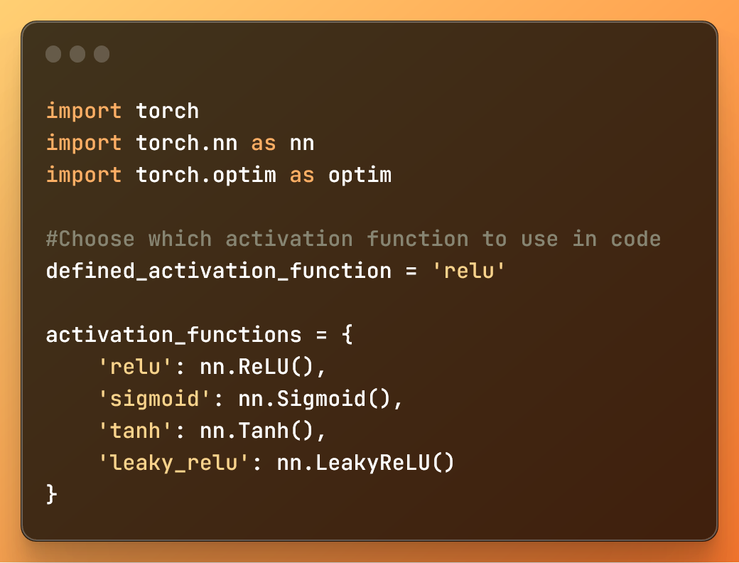 Importing libraries and defining dictionary with activation functions
In this code:
import torch: Imports the PyTorch library.import torch.nn as nn: Imports the neural network module from PyTorch.import torch.optim as optim: Imports the optimization module from PyTorch.
The variable and the dictionary above help you easily define, for this deep learning model, the activation function you want to use.
2: Defining hyperparameters and generating a dataset
# Initializing hyperparameters
num_samples = 100
batch_size = 10
num_epochs = 150
learning_rate = 0.001

# Define a simple synthetic dataset
def generate_data(num_samples):
    X = torch.randn(num_samples, 10)
    y = torch.randn(num_samples, 1)
    return X, y

# Generate synthetic data
X, y = generate_data(num_samples)
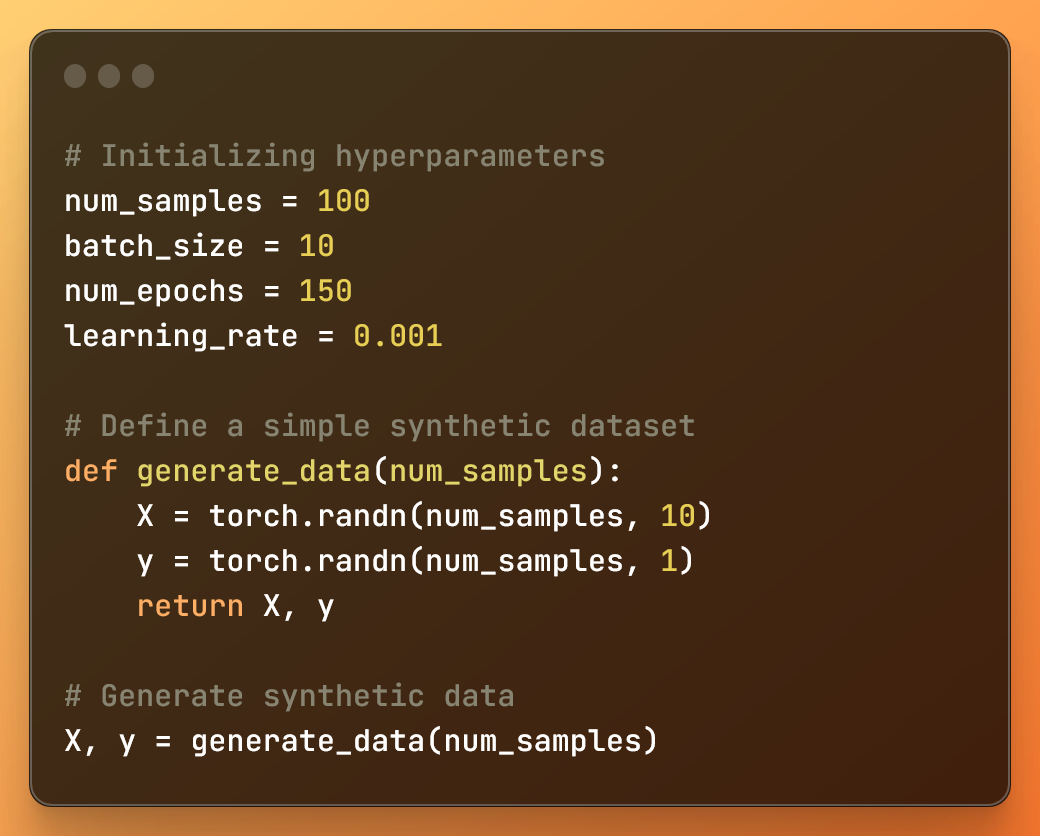 Initializing hyperparameters and creating, with a function, a synthetic dataset
In this code:
num_samplesis the number of samples in the synthetic dataset.batch_sizeis the size of each mini-batch during training.num_epochsis the number of iterations over the entire dataset during training.learning_rateis the learning rate used by the optimization algorithm.
Besides, we define a generate_data function to create two tensors with random values. Then it calls the function and it generates, for X and y, two tensors with random values.
3: Creating the deep learning model
class SimpleModel(nn.Module):
    def __init__(self, activation=defined_activation_function):
        super(SimpleModel, self).__init__()
        self.fc1 = nn.Linear(in_features=10, out_features=18)
        self.fc2 = nn.Linear(in_features=18, out_features=18)
        self.fc3 = nn.Linear(in_features=18, out_features=4)
        self.fc4 = nn.Linear(in_features=4, out_features=1)
        self.activation = activation_functions[activation]

    def forward(self, x):
        x = self.fc1(x)
        x = self.activation(x)
        x = self.fc2(x)
        x = self.activation(x)
        x = self.fc3(x)
        x = self.activation(x)
        x = self.fc4(x)
        return x
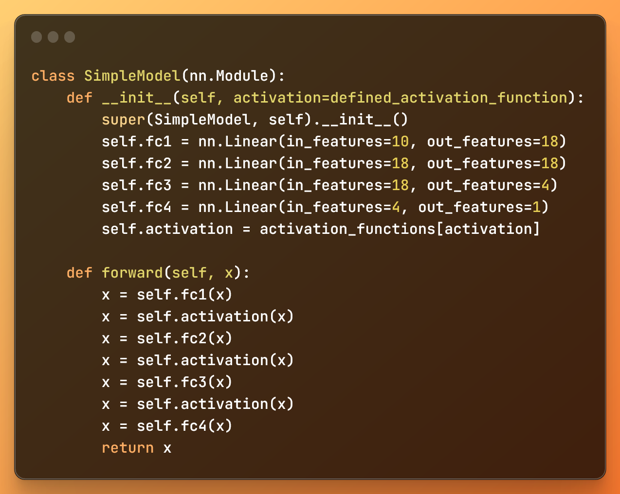 A simple feed forward neural network deep learning AI model
The __init__ method in the SimpleModel class initializes the neural network architecture. It initializes four fully connected layers and defines the activation function we are going to use.
We create each layer using nn.Linear, while the forward method defines how the data flows through the neural network.
4: Initializing the model and defining the loss function and optimizer
model = SimpleModel(activation=defined_activation_function)
criterion = nn.MSELoss()
optimizer = optim.Adam(model.parameters(), lr=learning_rate)
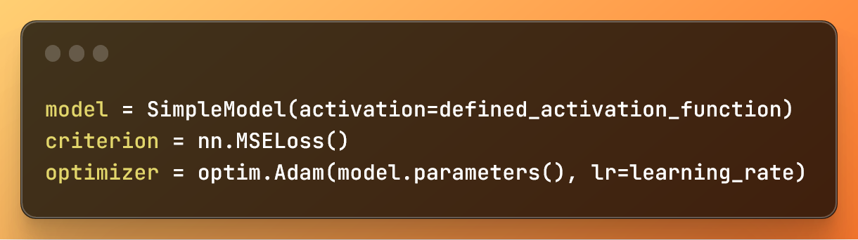 Defining activation function, loss function and gradient descend variation to be used
In this code:
model = SimpleModel(activation=defined_activation_function)creates a neural network model with a specified activation function.criterion = nn.MSELoss()defines the Mean Squared Error (MSE) Loss function.optimizer = optim.Adam(model.parameters(), lr=learning_rate)sets up the Adam optimizer for updating the model parameters during training, with a specified learning rate.
5: Training the deep learning model
for epoch in range(num_epochs):
    for i in range(0, num_samples, batch_size):
        # Get the mini-batch
        inputs = X[i:i+batch_size]
        labels = y[i:i+batch_size]

        # Zero the parameter gradients
        optimizer.zero_grad()

        # Forward pass
        outputs = model(inputs)

        # Compute the loss
        loss = criterion(outputs, labels)

        # Backward pass and optimize
        loss.backward()
        optimizer.step()

    print(f'Epoch {epoch+1}/{num_epochs}, Loss: {loss}')
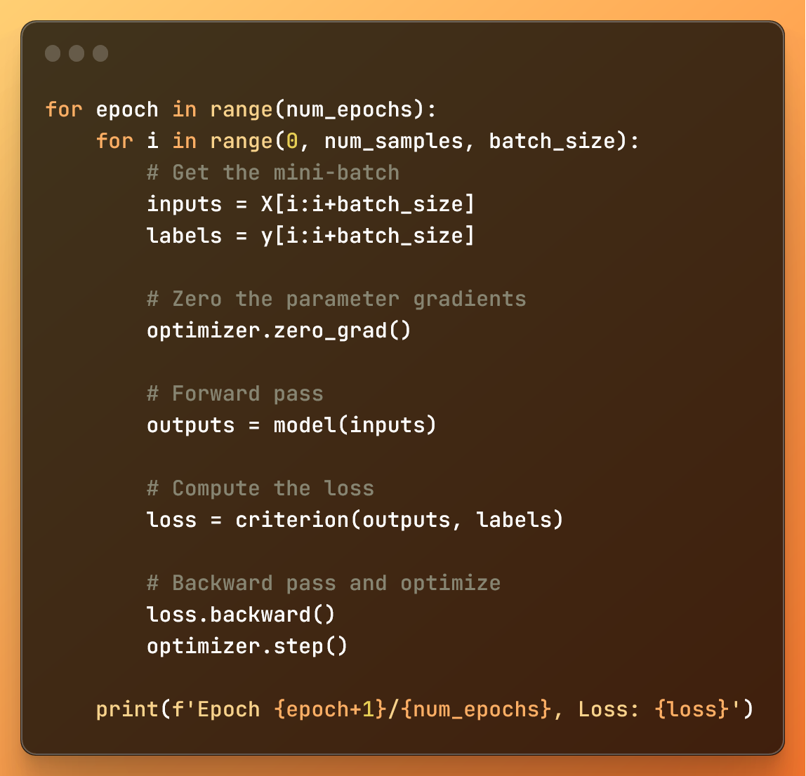 Training the model
- The outer loop, based on
num_epochs(number of epochs) controls how many times the entire dataset is processed. - The inner loop divides the dataset in mini-batches using the range function.
In each mini loop:
- With inputs and labels, we get the data from the mini-batch we want to process
- We eliminate with
optimizer.zero_grad(), the gradients – variables that tell us how to adjust weights for accurate predictions – of the previous mini-batch iteration. This is important to prevent mixing gradient information between mini-batches. - The forward pass gets us the model predictions (
outputs), and the loss is calculated using the specified loss function (criterion). - With
loss.backward(), we calculate the gradients for the weights. - Finally,
optimizer.step()updates the model's weights based on those gradients to minimize the loss function.
This is the full code to train a very simple deep learning model on a very simple dataset.
It does not have anything more advanced like convolutional neural networks.
Conclusion: The Unsung Heroes of AI Neural Networks
Activation functions are like gatekeepers. By restricting the flow of information, the neural network can learn better.
Activation functions are just like people when they study, or soccer players when deciding what to do with a ball.
These functions give neural networks the ability to learn and predict correctly.
Mathematically, activation functions are what allow the correct approximation of any linear or non-linear function in neural networks. Without them, neural networks approximate only linear functions.
And I leave you with this:
The mathematical idea of a neural network being able to approximate any non linear function is called the Universal Approximation Theorem.
You can find the full code on GitHub here: