
A Vigenère Cipher encrypts and decrypts text using a different alphabet for each letter. It consists of text to encrypt and a key with a different letter corresponding to each letter in the text.
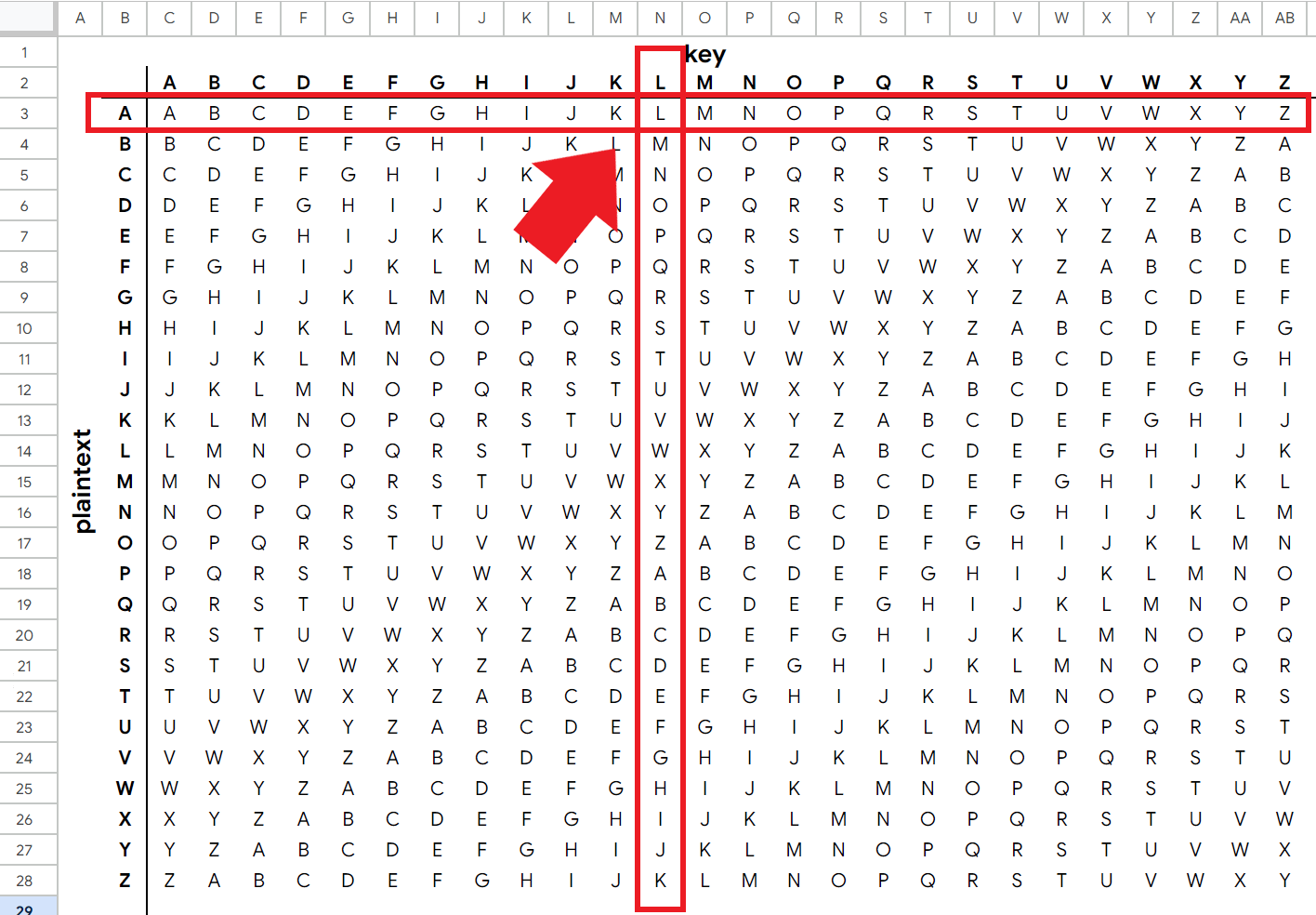
Creating a grid of alphabets helps illustrate this practice. If the first letter in your text is A and the first letter in your key is L, you would find the encrypted letter, L, where the plaintext and key intersect:
 screenshot of a grid of alphabets
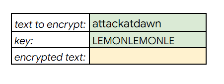
So your text to encrypt might look like this: attackatdawn, your key might be this: LEMONLEMONLE, and the ciphertext would be this: LXFOPVEFRNHR.
This is the same example used on the Wikipedia page which I'll walk you through in this article.
You could create a cipher encoder/decoder with any number of programming languages. But spreadsheets are a nice tool to use for this kind of project because they come with some pretty robust built-in functions that will help us dissect the cipher.
I've chosen Google Sheets because it's a hair simpler to jump into, especially if you already have a Gmail account. But you can do all the same things in Microsoft Excel.
Here's the Google Sheet I used.
If you'd like to check out a video walkthrough, here you go 👇
Spreadsheet Preparation
This isn't too complicated. We need a grid of alphabets. No, you don't have to type them in over and over, either.
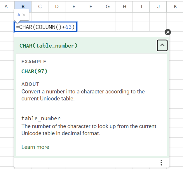
In fact, you don't even have to type the whole first alphabet. Let's use Unicode characters. For capital letters, the Unicode for the alphabet starts with 65.
The CHAR() function in spreadsheets converts a number into a character according to the current Unicode table.
The COLUMN() function returns a number corresponding to the current column where column A returns 1, column B returns 2, and so on.
So if we start our alphabet in column B, we can access each letter by adding 63 to the COLUMN() function and wrapping it in the CHAR() function:
=CHAR(COLUMN()+63)
Then we can drag this over to the right until we've got the full alphabet.
 screenshot of CHAR and COLUMN functions
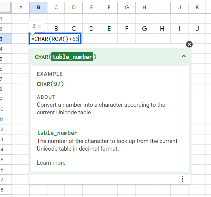
The same thing applies going down. We'll just use the ROW() function instead:
=CHAR(ROW()+63)
 screenshot of CHAR and ROW functions
Then we can reference the cell above and to the right for every cell below to fill out the full alphabet grid:
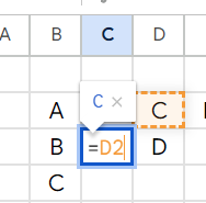 screenshot of spreadsheet cell
The only one that will be different will be in the last column where we'll need to reference the first column to have the alphabet wrap:
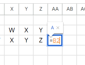 screenshot of spreadsheet cell
We only have to do this on the second line. Then, select the full second row and drag the formulas down to fill out the grid:
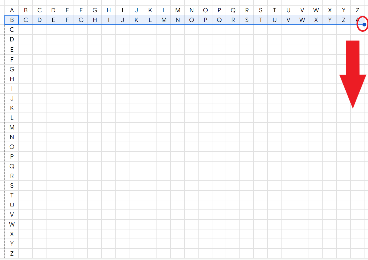 screenshot of spreadsheet grid
At this point, you can copy CTRL + C and paste values only CTRL + SHIFT + V for all the alphabet. If you add or shift rows, the alphabets may get skewed since their formulas reference fixed columns.
The Game Plan
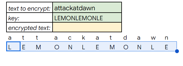
Now the fun stuff. We want our text to be encrypted automatically. Let's highlight three cells: one for the text to encrypt, one for a key, and then a blank cell for our encrypted text:
 screenshot of text to encrypt
Note: the key needs to be the same length as the text to encrypt/decrypt. In this example, the key is the word LEMON, but we extend it by repeating it for every character we need to encrypt.
Now we need to do three things:
- Split out each character of our text into its own cell
- Loop through each character and encrypt it based on the corresponding key character.
- Join all those characters together and place the result in our encrypted text cell.
Split Text to Setup
Interestingly, we cannot use the SPLIT() - or if you're in Excel, the TEXTSPLIT() - function without a delimiter. That is, we can't just tell it to split each character without there being something in between the characters.
So, we have to get fancy. In the video walkthrough, I explore a Google Sheets-specific approach using regular expressions...which are hard fun.
Here's what it looks like, and it involves creating character groups, inserting something in between each one, and then splitting using that same something as the delimiter. I used a blank space as the thing which I inserted and then split by:
=SPLIT(REGEXREPLACE(AG6,"(.)","$1 ")," ")
 gif of woman saying, that's just hard
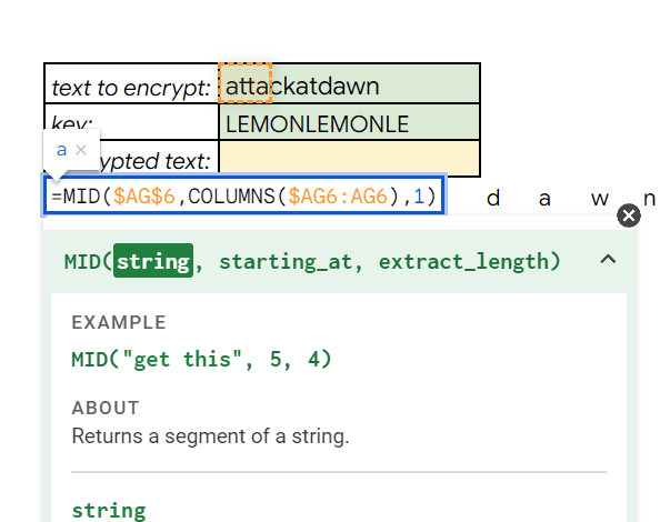
Excel users and mortals, fear not – there's a more elegant way that I'll show you here that can be done in either program by using the MID() and COLUMNS() functions.
The MID() function extracts a segment of a string, and COLUMNS() returns the number of columns in an array. By nesting COLUMNS() inside MID() we can one by one extract each character from the string:
=MID($AG$6,COLUMNS($AG6:AG6),1)
 screenshot of MID and COLUMNS functions
By locking $AG6 as the first part of the array referenced in the COLUMNS() function, this number adds one for every column we drag our formula over.
Drag this over until you reach the end of the text to encrypt. Every character should be in its own cell now. Do the same for the key.
 screenshot of spreadsheet cells
How to Use XLOOKUP() to Encrypt
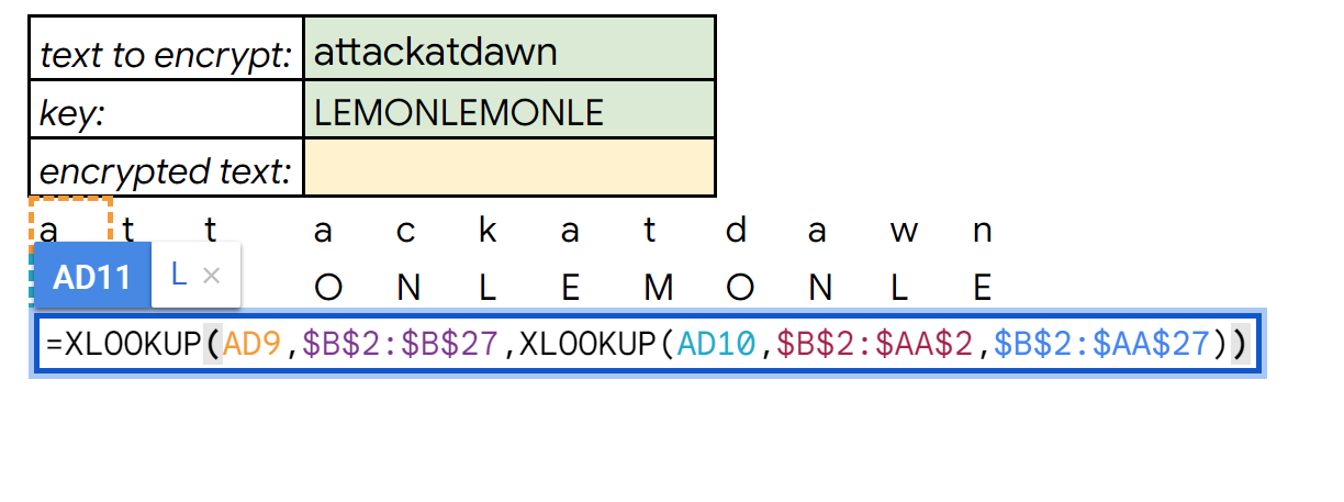
Below each pairing of plaintext and key text, we will now do a double XLOOKUP().
Yes, it's as awesome as it sounds.
Here's what it looks like, and let's walkthrough what's happening:
=XLOOKUP(AD9,$B$2:$B$27,XLOOKUP(AD10,$B$2:$AA$2,$B$2:$AA$27))
 screenshot of double XLOOKUP functions
For the beginning XLOOKUP(), we are looking up the plaintext and we're referencing the first plaintext alphabet for our lookup range. But then for our result range, we're opening up another XLOOKUP()...
This is because we still have to use the correct key alphabet to return an encrypted value.
So, we need the second XLOOKUP() to return a full alphabet based on the position of the key character.
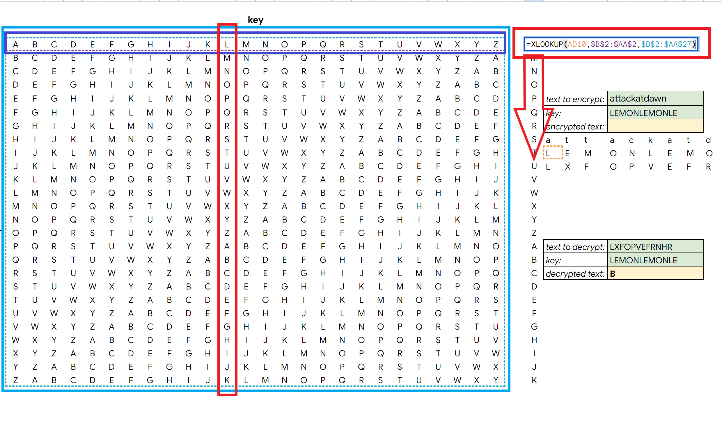
We're using the key character as our lookup value, we're using the first alphabet along the top key row for our lookup range, and then we're returning the whole grid as our result range. This will let us return a full alphabet which is in turn referenced as the result range for our first XLOOKUP().
 screenshot of alphabet grid and XLOOKUP example
You can see the second XLOOKUP() by itself in the picture above. The formula is in the top left. We're using the first letter of key text as the lookup value. The lookup range is the top alphabet in the purple box. The result range is the whole grid in the blue box. And the returned alphabet is the one that starts with L in the red box.
You can see it being returned underneath the formula where there is an arrow in the picture.
Drag the double XLOOKUP() function over to encrypt every character of the plaintext with the key text.
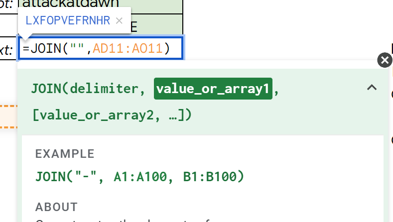
Join Text for Final Solution
Now that we've encrypted each letter, we want them to be joined into one string and returned in our encrypted text cell.
To do this, we can use the JOIN() function - or TEXTJOIN() for Excel - with an empty quote as the delimiter.
=JOIN("",AD11:AO11)
 screenshot of JOIN function
And voilà! We've just encrypted a string using a double XLOOKUP().
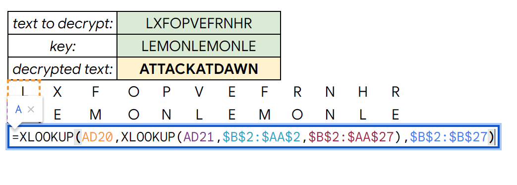
How to Decrypt Text
Decryption works exactly the same. The only difference is the placement of the second XLOOKUP(). Instead of using it as the result range, we're using it as the lookup range:
=XLOOKUP(AD20,XLOOKUP(AD21,$B$2:$AA$2,$B$2:$AA$27),$B$2:$B$27)
 screenshot of decryption double XLOOKUP example
Thanks for reading
I hope this was helpful for you and that you learned something new!
You can find more of my tutorials on YouTube, and please sign up for my newsletter about coding and spreadsheets here.