
Technology has become an asset in finance. Financial institutions are now evolving into technology companies rather than just staying occupied with the financial aspects of the field.
Mathematical Algorithms bring about innovation and speed. They can help us gain a competitive advantage in the market.
The speed and frequency of financial transactions, together with the large data volumes, has drawn a lot of attention towards technology from all the big financial institutions.
Algorithmic or Quantitative trading is the process of designing and developing trading strategies based on mathematical and statistical analyses. It is an immensely sophisticated area of finance.
This tutorial serves as the beginner’s guide to quantitative trading with Python. You’ll find this post very helpful if you are:
A student or someone aiming to become a quantitative analyst (quant) at a fund or bank.
Someone who is planning to start their own quantitative trading business.
We’ll go over the following topics in this post:
Basics of stocks and trading
Extracting data from Quandl API
Exploratory data analysis on stock pricing data
Moving averages
Formulating a trading strategy with Python
Visualizing the performance of the strategy
Before we deep dive into the details and dynamics of stock pricing data, we must first understand the basics of finance. If you are someone who is familiar with finance and how trading works, you can skip this section and click here to go to the next one.
What Are Stocks? What is Stock Trading?
Stocks
A stock is a representation of a share in the ownership of a corporation, which is issued at a certain amount. It is a type of financial security that establishes your claim on a company’s assets and performance.
An organization or company issues stocks to raise more funds/capital in order to scale and engage in more projects. These stocks are then publicly available and are sold and bought.
Stock Trading and Trading Strategy
The process of buying and selling existing and previously issued stocks is called stock trading. There is a price at which a stock can be bought and sold, and this keeps on fluctuating depending upon the demand and the supply in the share market.
Depending on the company’s performance and actions, stock prices may move up and down, but the stock price movement is not limited to the company’s performance.
Traders pay money in return for ownership within a company, hoping to make some profitable trades and sell the stocks at a higher price.
Another important technique that traders follow is short selling . This involves borrowing shares and immediately selling them in the hope of buying them up later at a lower price, returning them to the lender, and making the margin.
So, most traders follow a plan and model to trade. This is known as a trading strategy.
Quantitative traders at hedge funds and investment banks design and develop these trading strategies and frameworks to test them. It requires profound programming expertise and an understanding of the languages needed to build your own strategy.
Python is one of the most popular programming languages used, among the likes of C++, Java, R, and MATLAB. It is being adopted widely across all domains, especially in data science, because of its easy syntax, huge community, and third-party support.
You’ll need familiarity with Python and statistics in order to make the most of this tutorial. Make sure to brush up on your Python and check out the fundamentals of statistics.
Extracting data from the Quandl API
In order to extract stock pricing data, we’ll be using the Quandl API. But before that, let’s set up the work environment. Here’s how:
- In your terminal, create a new directory for the project (name it however you want):
mkdir <directory_name>
Make sure you have Python 3 and virtualenv installed on your machine.
Create a new Python 3 virtualenv using
virtualenv <env_name>and activate it usingsource <env_name>/bin/activate.Now, install jupyter-notebook using pip, and type in
pip install jupyter-notebookin the terminal.Similarly, install the
pandas,quandl, andnumpypackages.Run your
jupyter-notebookfrom the terminal.
Now, your notebook should be running on localhost like the screenshot below:

You can create your first notebook by clicking on the New dropdown on the right. Make sure you have created an account on Quandl. Follow the steps mentioned here to create your API key.
Once you’re all set, let’s dive right in:
# importing required packages
import pandas as pd
import quandl as q
Pandas is going to be the most rigorously used package in this tutorial as we’ll be doing a lot of data manipulation and plotting.
After the packages are imported, we will make requests to the Quandl API by using the Quandl package:
# set the API key
q.ApiConfig.api_key = "<API key>”
#send a get request to query Microsoft's end of day stock prices from 1st #Jan, 2010 to 1st Jan, 2019

msft_data = q.get("EOD/MSFT", start_date="2010-01-01", end_date="2019-01-01")
# look at the first 5 rows of the dataframe

msft_data.head()

Here we have Microsoft’s EOD stock pricing data for the last 9 years. All you had to do was call the get method from the Quandl package and supply the stock symbol, MSFT, and the timeframe for the data you need.
This was really simple, right? Let’s move ahead to understand and explore this data further.
Exploratory Data Analysis on Stock Pricing Data
With the data in our hands, the first thing we should do is understand what it represents and what kind of information it encapsulates.
Printing the DataFrame’s info, we can see all that it contains:
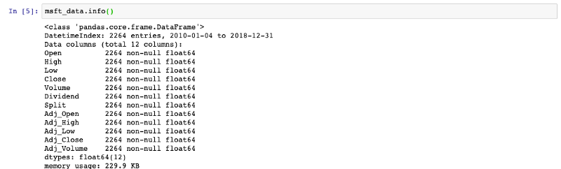
As seen in the screenshot above, the DataFrame contains DatetimeIndex, which means we’re dealing with time-series data.
An index can be thought of as a data structure that helps us modify or reference the data. Time-series data is a sequence of snapshots of prices taken at consecutive, equally spaced intervals of time.
In trading, EOD stock pricing data captures the movement of certain parameters about a stock, such as the stock price, over a specified period of time with data points recorded at regular intervals.
Important Terminology
Looking at other columns, let’s try to understand what each column represents:
Open/Close — Captures the opening/closing price of the stock
Adj_Open/Adj_Close — An adjusted opening/closing price is a stock’s price on any given day of trading that has been revised to include any dividend distributions, stock splits, and other corporate actions that occurred at any time before the next day’s open.
Volume — It records the number of shares that are being traded on any given day of trading.
High/Low — It tracks the highest and the lowest price of the stock during a particular day of trading.
These are the important columns that we will focus on at this point in time.
We can learn about the summary statistics of the data, which shows us the number of rows, mean, max, standard deviations, and so on. Try running the following line of code in the Ipython cell:
msft_data.describe()

resample()
Pandas’ resample() method is used to facilitate control and flexibility on the frequency conversion of the time series data. We can specify the time intervals to resample the data to monthly, quarterly, or yearly, and perform the required operation over it.
msft_data.resample('M').mean()
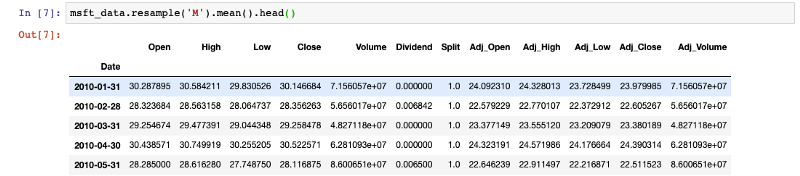
This is an interesting way to analyze stock performance in different timeframes.
Calculating returns
A financial return is simply the money made or lost on an investment. A return can be expressed nominally as the change in the amount of an investment over time. It can be calculated as the percentage derived from the ratio of profit to investment.
We have the pct_change() at our disposal for this purpose. Here is how you can calculate returns:
# Import numpy package
import numpy as np
# assign `Adj Close` to `daily_close`
daily_close = msft_data[['Adj_Close']]
# returns as fractional change
daily_return = daily_close.pct_change()
# replacing NA values with 0

daily_return.fillna(0, inplace=True)
print(daily_return)
This will print the returns that the stock has been generating on a daily basis. Multiplying the number by 100 will give you the percentage change.
The formula used in pct_change() is:
Return = {(Price at t) — (Price at t-1)} / {Price at t-1}
Now, to calculate monthly returns, all you need to do is:
mdata = msft_data.resample('M').apply(lambda x: x[-1])

monthly_return = mdata.pct_change()
After resampling the data to months (for business days), we can get the last day of trading in the month using the apply() function.
apply() takes in a function and applies it to each and every row of the Pandas series. The lambda function is an anonymous function in Python which can be defined without a name, and only takes expressions in the following format:
Lambda: expression
For example, lambda x: x * 2 is a lambda function. Here, x is the argument and x * 2 is the expression that gets evaluated and returned.
Moving Averages in Trading
The concept of moving averages is going to build the base for our momentum-based trading strategy.
In finance, analysts often have to evaluate statistical metrics continually over a sliding window of time, which is called moving window calculations.
Let’s see how we can calculate the rolling mean over a window of 50 days, and slide the window by 1 day.
rolling()
This is the magical function which does the tricks for us:
# assigning adjusted closing prices to

adj_pricesadj_price = msft_data['Adj_Close']
# calculate the moving average
mav = adj_price.rolling(window=50).mean()
# print the resultprint(mav[-10:])

You’ll see the rolling mean over a window of 50 days (approx. 2 months). Moving averages help smooth out any fluctuations or spikes in the data, and give you a smoother curve for the performance of the company.
We can plot and see the difference:
# import the matplotlib package to see the plot

import matplotlib.pyplot as plt

adj_price.plot()

You can now plot the rolling mean():
mav.plot()

And you can see the difference for yourself, how the spikes in the data are consumed to give a general sentiment around the performance of the stock.
Formulating a Trading Strategy
Here comes the final and most interesting part: designing and making the trading strategy. This will be a step-by-step guide to developing a momentum-based Simple Moving Average Crossover (SMAC) strategy.
Momentum-based strategies are based on a technical indicator that capitalizes on the continuance of the market trend. We purchase securities that show an upwards trend and short-sell securities which show a downward trend.
The SMAC strategy is a well-known schematic momentum strategy. It is a long-only strategy. Momentum, here, is the total return of stock including the dividends over the last n months. This period of n months is called the lookback period.
There are 3 main types of lookback periods: short term, intermediate-term, and long term. We need to define 2 different lookback periods of a particular time series.
A buy signal is generated when the shorter lookback rolling mean (or moving average) overshoots the longer lookback moving average. A sell signal occurs when the shorter lookback moving average dips below the longer moving average.
Now, let’s see how the code for this strategy will look:
# step1: initialize the short and long lookback periods

short_lb = 50long_lb = 120
# step2: initialize a new DataFrame called signal_df with a signal column

signal_df = pd.DataFrame(index=msft_data.index)signal_df['signal'] = 0.0
# step3: create a short simple moving average over the short lookback period
signal_df['short_mav'] = msft_data['Adj_Close'].rolling(window=short_lb,                                     min_periods=1, center=False).mean()
# step4: create long simple moving average over the long lookback period

signal_df['long_mav'] = msft_data['Adj_Close'].rolling(window=long_lb, min_periods=1, center=False).mean()
# step5: generate the signals based on the conditional statement

signal_df['signal'][short_lb:] = np.where(signal_df['short_mav'][short_lb:] > signal_df['long_mav'][short_lb:], 1.0, 0.0)
# step6: create the trading orders based on the positions column

signal_df['positions'] = signal_df['signal'].diff()signal_df[signal_df['positions'] == -1.0]
Let’s see what’s happening here. We have created 2 lookback periods. The short lookback period short_lb is 50 days, and the longer lookback period for the long moving average is defined as a long_lb of 120 days.
We have created a new DataFrame which is designed to capture the signals. These signals are being generated whenever the short moving average crosses the long moving average using the np.where. It assigns 1.0 for true and 0.0 if the condition comes out to be false.
The positions columns in the DataFrame tells us if there is a buy signal or a sell signal, or to stay put. We're basically calculating the difference in the signals column from the previous row using diff.
And there we have our strategy implemented in just 6 steps using Pandas. Easy, wasn't it?
Now, let’s try to visualize this using Matplotlib. All we need to do is initialize a plot figure, add the adjusted closing prices, short, and long moving averages to the plot, and then plot the buy and sell signals using the positions column in the signal_df above:
# initialize the plot using plt
fig = plt.figure()
# Add a subplot and label for y-axis

plt1 = fig.add_subplot(111,  ylabel='Price in $')
msft_data['Adj_Close'].plot(ax=plt1, color='r', lw=2.)
# plot the short and long lookback moving averages
signal_df[['short_mav', 'long_mav']].plot(ax=plt1, lw=2., figsize=(12,8))
# plotting the sell signals

plt1.plot(signal_df.loc[signal_df.positions == -1.0].index,                         signal_df.short_mav[signal_df.positions == -1.0],'v',                     markersize=10, color='k')
# plotting the buy signals

plt1.plot(signal_df.loc[signal_df.positions == 1.0].index,          signal_df.short_mav[signal_df.positions == 1.0],         '^', markersize=10, color='m')         # Show the plotplt.show()
Running the above cell in the Jupyter notebook would yield a plot like the one below:

Now, you can clearly see that whenever the blue line (short moving average) goes up and beyond the orange line (long moving average), there is a pink upward marker indicating a buy signal.
A sell signal is denoted by a black downward marker where there’s a fall of the short_mav below long_mav.
Visualize the Performance of the Strategy on Quantopian
Quantopian is a Zipline-powered platform that has manifold use cases. You can write your own algorithms, access free data, backtest your strategy, contribute to the community, and collaborate with Quantopian if you need capital.
We have written an algorithm to backtest our SMA strategy, and here are the results:
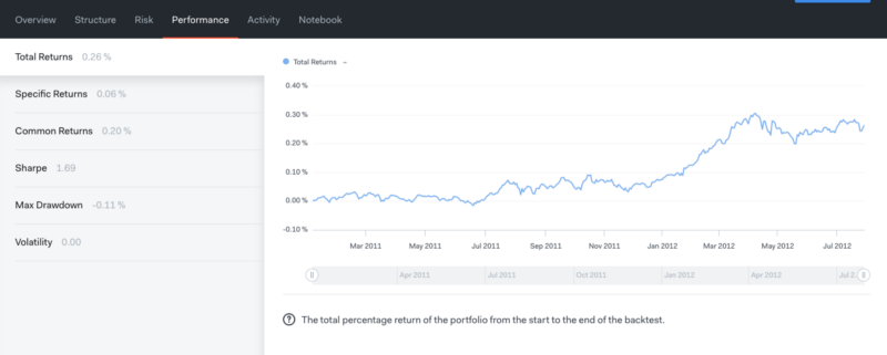
Here is an explanation of the above metrics:
Total return: The total percentage return of the portfolio from the start to the end of the backtest.
Specific return: The difference between the portfolio’s total returns and common returns.
Common return: Returns that are attributable to common risk factors. There are 11 sector and 5 style risk factors that make up these returns. The Sector Exposure and Style Exposure charts in the Risk section provide more detail on these factors.
Sharpe: The 6-month rolling Sharpe ratio. It is a measure of risk-adjusted investment. It is calculated by dividing the portfolio’s excess returns over the risk-free rate by the portfolio’s standard deviation.
Max Drawdown: The largest drop of all the peak-to-trough movement in the portfolio’s history.
Volatility: Standard deviation of the portfolio’s returns.
Pat yourself on the back as you have successfully implemented your quantitative trading strategy!
Where to go From Here?
Now that your algorithm is ready, you’ll need to backtest the results and assess the metrics mapping the risk involved in the strategy and the stock. Again, you can use BlueShift and Quantopian to learn more about backtesting and trading strategies.
Further Resources
![]()
https://quantra.quantinsti.com/learning-track/algorithmic-trading-for-everyone?utm_source=harshit_tyagi&utm_medium=affiliate&utm_campaign=lt_everyone
Quantra is a brainchild of QuantInsti. With a range of free and paid courses by experts in the field, Quantra offers a thorough guide on a bunch of basic and advanced trading strategies.
Data Science Course — They have rolled out an introductory course on Data Science that helps you build a strong foundation for projects in Data Science.
Trading Courses for Beginners — From momentum trading to machine and deep learning-based trading strategies, researchers in the trading world like Dr. Ernest P. Chan are the authors of these niche courses.
Free Resources
To learn more about trading algorithms, check out these blogs:
Quantstart — they cover a wide range of backtesting algorithms, beginner guides, and more.
Investopedia — everything you want to know about investment and finance.
Quantivity — detailed mathematical explanations of algorithms and their pros and cons.
Warren Buffet says he reads about 500 pages a day, which should tell you that reading is essential in order to succeed in the field of finance.
Embark upon this journey of trading and you can lead a life full of excitement, passion, and mathematics.
Data Science with Harshit
With this channel, I am planning to roll out a couple of series covering the entire data science space. Here is why you should be subscribing to the channel:
These series would cover all the required/demanded quality tutorials on each of the topics and subtopics like Python fundamentals for Data Science.
Explained Mathematics and derivations of why we do what we do in ML and Deep Learning.
Podcasts with Data Scientists and Engineers at Google, Microsoft, Amazon, etc, and CEOs of big data-driven companies.
Projects and instructions to implement the topics learned so far. Learn about new certifications, Bootcamp, and resources to crack those certifications like this TensorFlow Developer Certificate Exam by Google.
If this tutorial was helpful, you should check out my data science and machine learning courses on Wiplane Academy. They are comprehensive yet compact and helps you build a solid foundation of work to showcase.