An intuitive introduction to Generative Adversarial Networks (GANs)

by Thalles Silva

Warm up

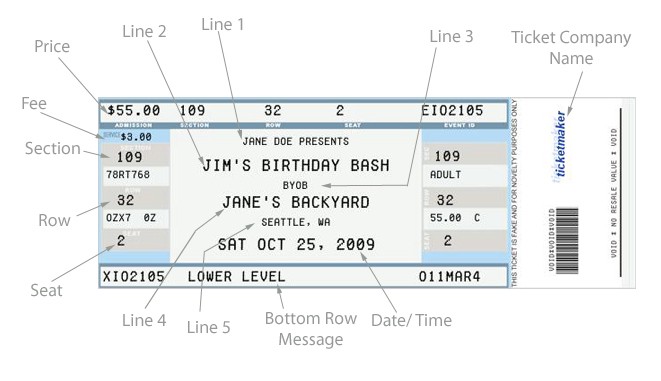
Let’s say there’s a very cool party going on in your neighborhood that you really want to go to. But, there is a problem. To get into the party you need a special ticket — that was long sold out.

Wait up! Isn’t this a Generative Adversarial Networks article? Yes it is. But bear with me for now, it is going to be worth it.

OK, since expectations are very high, the party organizers hired a qualified security agency. Their primary goal is to not allow anyone to crash the party. To do that, they placed a lot of guards at the venue’s entrance to check everyone’s tickets for authenticity.

Since you don’t have any martial artistic gifts, the only way to get through is by fooling them with a very convincing fake ticket.

There is a big problem with this plan though — you never actually saw how the ticket looks like.

Even if you design a ticket based on your creativity, it’s almost impossible to fool the guards at your first trial. Besides, you can’t show your face until you have a very decent replica of the party’s pass.

To help solve the problem, you decide to call your friend Bob to do the job for you.

Bob’s mission is very simple. He will try to get into the party with your fake pass. If he gets denied, he will come back to you with useful tips on how the ticket should look like.

Based on that feedback, you make a new version of the ticket and hand it to Bob, who goes to try again. This process keeps repeating until you become able to design a perfect replica.

Putting aside the ‘small holes’ in this anecdote, this is pretty much how Generative Adversarial Networks (GANs) work.

Nowadays, most of the applications of GANs are in the field of computer vision. Some of the applications include training semi-supervised classifiers, and generating high resolution images from low resolution counterparts.

This piece provides an introduction to GANs with a hands-on approach to the problem of generating images. You can clone the notebook for this post here.

Generative Adversarial Networks

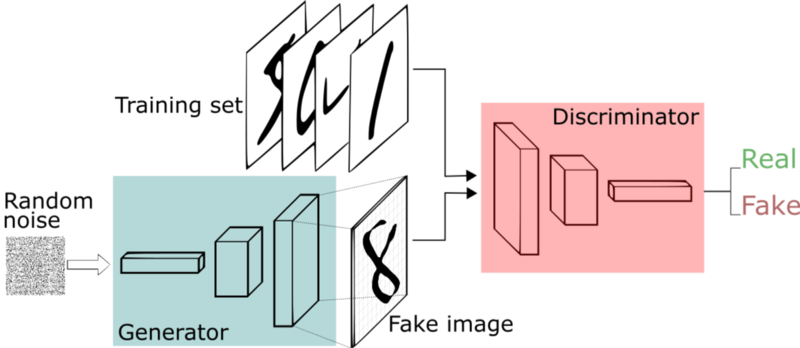
GANs are generative models devised by Goodfellow et al. in 2014. In a GAN setup, two differentiable functions, represented by neural networks, are locked in a game. The two players (the generator and the discriminator) have different roles in this framework.

The generator tries to produce data that come from some probability distribution. That would be you trying to reproduce the party’s tickets.

The discriminator acts like a judge. It gets to decide if the input comes from the generator or from the true training set. That would be the party’s security comparing your fake ticket with the true ticket to find flaws in your design.

In summary, the game follows with:

• The generator trying to maximize the probability of making the discriminator mistakes its inputs as real.
• And the discriminator guiding the generator to produce more realistic images.

In the perfect equilibrium, the generator would capture the general training data distribution. As a result, the discriminator would be always unsure of whether its inputs are real or not.

In the DCGAN paper, the authors describe the combination of some deep learning techniques as key for training GANs. These techniques include: (i) the all convolutional net and (ii) Batch Normalization (BN).

The first emphasizes strided convolutions (instead of pooling layers) for both: increasing and decreasing feature’s spatial dimensions. And the second normalizes the feature vectors to have zero mean and unit variance in all layers. This helps to stabilize learning and to deal with poor weight initialization problems.

Without further ado, let’s dive into the implementation details and talk more about GANs as we go. We present an implementation of a Deep Convolutional Generative Adversarial Network (DCGAN). Our implementation uses Tensorflow and follows some practices described in the DCGAN paper.

Generator

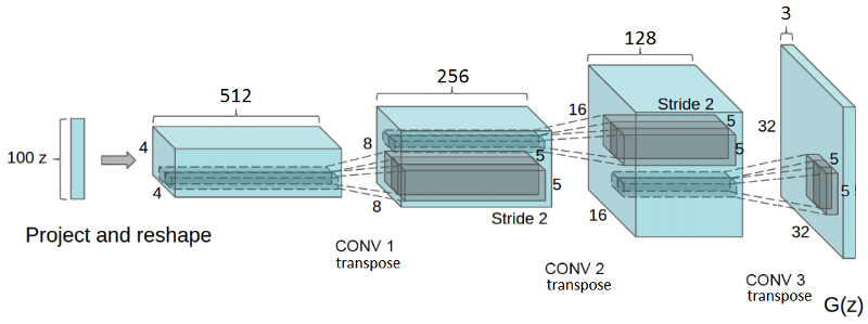
The network has 4 convolutional layers, all followed by BN (except for the output layer) and Rectified Linear unit (ReLU) activations.

It takes as an input a random vector z (drawn from a normal distribution). After reshaping z to have a 4D shape, we feed it to the generator that starts a series of upsampling layers.

Each upsampling layer represents a transpose convolution operation with strides 2. Transpose convolutions are similar to the regular convolutions.

Typically, regular convolutions go from wide and shallow layers to narrower and deeper ones. Transpose convolutions go the other way. They go from deep and narrow layers to wider and shallower.

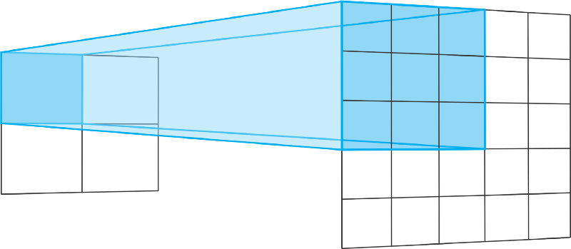
The stride of a transpose convolution operation defines the size of the output layer. With “same” padding and stride of 2, the output features will have double the size of the input layer.

That happens because, every time we move one pixel in the input layer, we move the convolution kernel by two pixels on the output layer. In other words, each pixel in the input image is used to draw a square in the output image.

In short, the generator begins with this very deep but narrow input vector. After each transpose convolution, z becomes wider and shallower. All transpose convolutions use a 5x5 kernel’s size with depths reducing from 512 all the way down to 3 — representing an RGB color image.

def transpose_conv2d(x, output_space):    return tf.layers.conv2d_transpose(x, output_space,       kernel_size=5, strides=2, padding='same',      kernel_initializer=tf.random_normal_initializer(mean=0.0,                                                      stddev=0.02))

The final layer outputs a 32x32x3 tensor — squashed between values of -1 and 1 through the Hyperbolic Tangent (tanh) function.

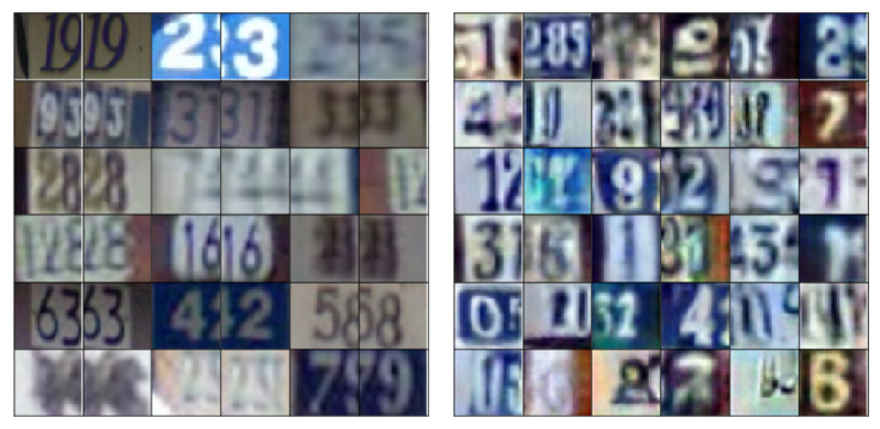
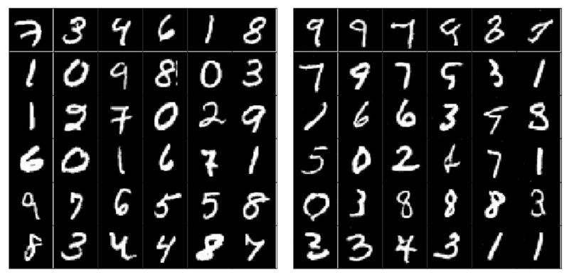
This final output shape is defined by the size of the training images. In this case, if training for SVHN, the generator produces 32x32x3 images. However, if training for MNIST, it would generate a 28x28 greyscale image.

Finally, note that before feeding the input vector z to the generator, we need to scale it to the interval of -1 to 1. That is to follow the choice of using the tanh function.

def generator(z, output_dim, reuse=False, alpha=0.2, training=True):    """    Defines the generator network    :param z: input random vector z    :param output_dim: output dimension of the network    :param reuse: Indicates whether or not the existing model variables should be used or recreated    :param alpha: scalar for lrelu activation function    :param training: Boolean for controlling the batch normalization statistics    :return: model's output    """    with tf.variable_scope('generator', reuse=reuse):        fc1 = dense(z, 4*4*512)        # Reshape it to start the convolutional stack        fc1 = tf.reshape(fc1, (-1, 4, 4, 512))        fc1 = batch_norm(fc1, training=training)        fc1 = tf.nn.relu(fc1)        t_conv1 = transpose_conv2d(fc1, 256)        t_conv1 = batch_norm(t_conv1, training=training)        t_conv1 = tf.nn.relu(t_conv1)        t_conv2 = transpose_conv2d(t_conv1, 128)        t_conv2 = batch_norm(t_conv2, training=training)        t_conv2 = tf.nn.relu(t_conv2)        logits = transpose_conv2d(t_conv2, output_dim)        out = tf.tanh(logits)        return out

Discriminator

The discriminator is also a 4 layer CNN with BN (except its input layer) and leaky ReLU activations. Many activation functions will work fine with this basic GAN architecture. However, leaky ReLUs are very popular because they help the gradients flow easier through the architecture.

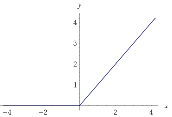
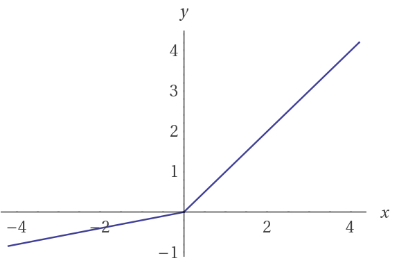
A regular ReLU function works by truncating negative values to 0. This has the effect of blocking the gradients to flow through the network. Instead of the function being zero, leaky ReLUs allow a small negative value to pass through. That is, the function computes the greatest value between the features and a small factor.

def lrelu(x, alpha=0.2):     # non-linear activation function    return tf.maximum(alpha * x, x)

Leaky ReLUs represent an attempt to solve the dying ReLU problem. This situation occurs when the neurons get stuck in a state in which ReLU units always output 0s for all inputs. For these cases, the gradients are completely shut to flow back through the network.

This is especially important for GANs since the only way the generator has to learn is by receiving the gradients from the discriminator.

The discriminator starts by receives a 32x32x3 image tensor. Opposite to the generator, the discriminator performs a series of strided 2 convolutions. Each, works by reducing the feature vector’s spatial dimensions by half its size, also doubling the number of learned filters.

Finally, the discriminator needs to output probabilities. For that, we use the Logistic Sigmoid activation function on the final logits.

def discriminator(x, reuse=False, alpha=0.2, training=True):    """    Defines the discriminator network    :param x: input for network    :param reuse: Indicates whether or not the existing model variables should be used or recreated    :param alpha: scalar for lrelu activation function    :param training: Boolean for controlling the batch normalization statistics    :return: A tuple of (sigmoid probabilities, logits)    """    with tf.variable_scope('discriminator', reuse=reuse):        # Input layer is 32x32x?        conv1 = conv2d(x, 64)        conv1 = lrelu(conv1, alpha)        conv2 = conv2d(conv1, 128)        conv2 = batch_norm(conv2, training=training)        conv2 = lrelu(conv2, alpha)        conv3 = conv2d(conv2, 256)        conv3 = batch_norm(conv3, training=training)        conv3 = lrelu(conv3, alpha)        # Flatten it        flat = tf.reshape(conv3, (-1, 4*4*256))        logits = dense(flat, 1)        out = tf.sigmoid(logits)        return out, logits

Note that in this framework, the discriminator acts as a regular binary classifier. Half of the time it receives images from the training set and the other half from the generator.

Back to our adventure, to reproduce the party’s ticket, the only source of information you had was the feedback from our friend Bob. In other words, the quality of the feedback Bob provided to you at each trial was essential to get the job done.

In the same way, every time the discriminator notices a difference between the real and fake images, it sends a signal to the generator. This signal is the gradient that flows backwards from the discriminator to the generator. By receiving it, the generator is able to adjust its parameters to get closer to the true data distribution.

This is how important the discriminator is. In fact, the generator will be as good as producing data as the discriminator is at telling them apart.

Losses

Now, let’s describe the trickiest part of this architecture — the losses. First, we know the discriminator receives images from both the training set and the generator.

We want the discriminator to be able to distinguish between real and fake images. Every time we run a mini-batch through the discriminator, we get logits. These are the unscaled values from the model.

However, we can divide the mini-batches that the discriminator receives in two types. The first, composed only with real images that come from the training set and the second, with only fake images — the ones created by the generator.

def model_loss(input_real, input_z, output_dim, alpha=0.2, smooth=0.1):    """    Get the loss for the discriminator and generator    :param input_real: Images from the real dataset    :param input_z: random vector z    :param out_channel_dim: The number of channels in the output image    :param smooth: label smothing scalar    :return: A tuple of (discriminator loss, generator loss)    """    g_model = generator(input_z, output_dim, alpha=alpha)    d_model_real, d_logits_real = discriminator(input_real, alpha=alpha)    d_model_fake, d_logits_fake = discriminator(g_model, reuse=True, alpha=alpha)    # for the real images, we want them to be classified as positives,      # so we want their labels to be all ones.    # notice here we use label smoothing for helping the discriminator to generalize better.    # Label smoothing works by avoiding the classifier to make extreme predictions when extrapolating.    d_loss_real = tf.reduce_mean(        tf.nn.sigmoid_cross_entropy_with_logits(logits=d_logits_real, labels=tf.ones_like(d_logits_real) * (1 - smooth)))    # for the fake images produced by the generator, we want the discriminator to clissify them as false images,    # so we set their labels to be all zeros.    d_loss_fake = tf.reduce_mean(        tf.nn.sigmoid_cross_entropy_with_logits(logits=d_logits_fake, labels=tf.zeros_like(d_model_fake)))    # since the generator wants the discriminator to output 1s for its images, it uses the discriminator logits for the    # fake images and assign labels of 1s to them.    g_loss = tf.reduce_mean(        tf.nn.sigmoid_cross_entropy_with_logits(logits=d_logits_fake, labels=tf.ones_like(d_model_fake)))    d_loss = d_loss_real + d_loss_fake    return d_loss, g_loss

Because both networks train at the same time, GANs also need two optimizers. Each one for minimizing the discriminator and generator’s loss functions respectively.

We want the discriminator to output probabilities close to 1 for real images and near 0 for fake images. To do that, the discriminator needs two losses. Therefore, the total loss for the discriminator is the sum of these two partial losses. One for maximizing the probabilities for the real images and another for minimizing the probability of fake images.

In the beginning of training two interesting situations occur. First, the generator does not know how to create images that resembles the ones from the training set. And second, discriminator does not know how to categorize the images it receives as real or fake.

As a result, the discriminator receives two very distinct types of batches. One, composed of true images from the training set and another containing very noisy signals. As training progresses, the generator starts to output images that look closer to the images from the training set. That happens, because the generator trains to learn the data distribution that composes the training set images.

At the same time, the discriminator starts to get real good at classifying samples as real or fake. As a consequence, the two types of mini-batches begin looking similar, in structure, to one another. That, as a result makes the discriminator unable to identify images as real or fake.

For the losses, we use vanilla cross-entropy with Adam as a good choice for the optimizer.

Concluding

GANs are one of the hottest subjects in machine learning right now. These models have the potential of unlocking unsupervised learning methods that would expand ML to new horizons.

Since its creation, researches have been developing many techniques for training GANs. In Improved Techniques for Training GANs, the authors describe state-of-the-art techniques for both image generation and semi-supervised learning.

If you are curious to dig deeper in these subjects, I recommend reading Generative Models.

Also, take a look at:

Dive head first into advanced GANs: exploring self-attention and spectral norm
Lately, Generative Models are drawing a lot of attention. Much of that comes from Generative Adversarial Networks…medium.freecodecamp.orgSemi-supervised learning with Generative Adversarial Networks (GANs)
If you ever heard or studied about deep learning, you probably heard about MNIST, SVHN, ImageNet, PascalVoc and others…towardsdatascience.com

And if you need more, that is my deep learning blog.

Enjoy, and thanks for reading!

Credits to Sam Williams for this awesome “clap” gif! Check it out in his post.