By Moshe Binieli
This article will explain you what Principal Component Analysis (PCA) is, why we need it and how we use it. I will try to make it as simple as possible while avoiding hard examples or words which can cause a headache.
A moment of honesty: to fully understand this article, a basic understanding of some linear algebra and statistics is essential. Take a few minutes to review the following topics, if you need to, in order to make it easy to understand PCA:
- vectors
- eigenvectors
- eigenvalues
- variance
- covariance
So how can this algorithm help us? What are the uses of this algorithm?
- Identifies the most relevant directions of variance in the data.
- Helps capture the most “important” features.
- Easier to make computations on the dataset after the dimension reductions since we have fewer data to deal with.
- Visualization of the data.
Short verbal explanation.
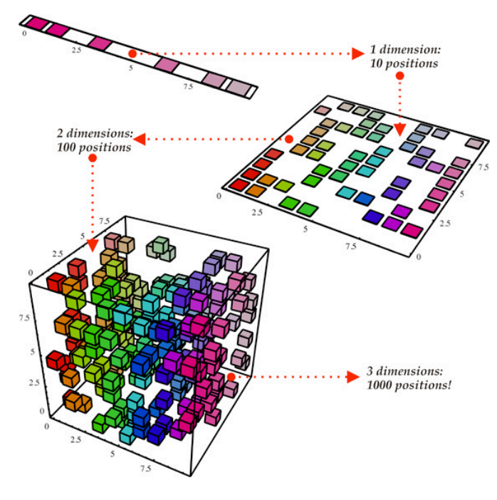
Let’s say we have 10 variables in our dataset and let’s assume that 3 variables capture 90% of the dataset, and 7 variables capture 10% of the dataset.
Let’s say we want to visualize 10 variables. Of course we cannot do that, we can visualize only maximum 3 variables (Maybe in future we will be able to).
So we have a problem: we don’t know which of the variables captures the largest variability in our data. To solve this mystery, we’ll apply the PCA Algorithm. The output will tell us who are those variables. Sounds cool, doesn’t it? ?
So what are the steps to make PCA work? How do we apply the magic?
- Take the dataset you want to apply the algorithm on.
- Calculate the covariance matrix.
- Calculate the eigenvectors and their eigenvalues.
- Sort the eigenvectors according to their eigenvalues in descending order.
- Choose the first K eigenvectors (where k is the dimension we’d like to end up with).
- Build new reduced dataset.
Time for an example with real data.
1) Load the dataset to a matrix:
Our main goal is to figure out how many variables are the most important for us and stay only with them.
For this example, we will use the program “Spyder” for running python. We’ll also use a pretty cool dataset that is embedded inside “sklearn.datasets” which is called “load_iris”. You can read more about this dataset at Wikipedia.
First of all, we will load the iris module and transform the dataset into a matrix. The dataset contains 4 variables with 150 examples. Hence, the dimensionality of our data matrix is: (150, 4).
import numpy as npimport pandas as pdfrom sklearn.datasets import load_iris
irisModule = load_iris()dataset = np.array(irisModule.data)
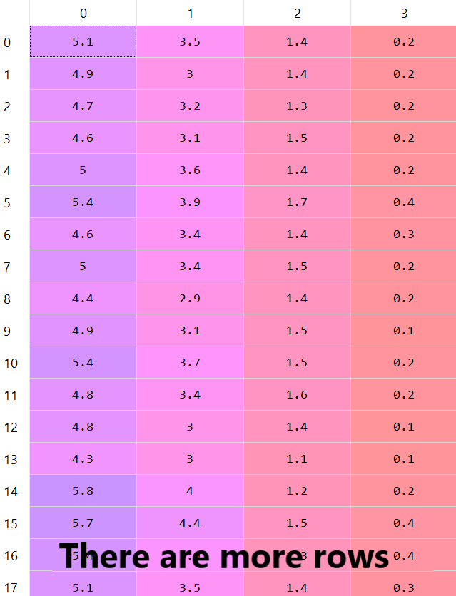
There are more rows in this dataset — as we said there are 150 rows, but we can see only 17 rows.
The concept of PCA is to reduce the dimensionality of the matrix by finding the directions that captures most of the variability in our data matrix. Therefore, we’d like to find them.
2) Calculate the covariance matrix:
It’s time to calculate the covariance matrix of our dataset, but what does this even mean? Why do we need to calculate the covariance matrix? How will it look?
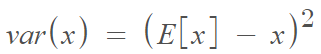
Variance is the expectation of the squared deviation of a random variable from its mean. Informally, it measures the spread of a set of numbers from their mean. The mathematical definition is:
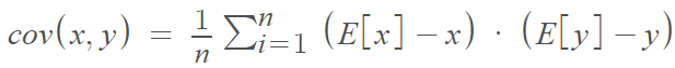
Covariance is a measure of the joint variability of two random variables. In other words, how any 2 features vary from each other. Using the covariance is very common when looking for patterns in data. The mathematical definition is:
From this definition, we can conclude that the covariance matrix will be symmetric. This is important because it means that its eigenvectors will be real and non-negative, which makes it easier for us (we dare you to claim that working with complex numbers is easier than real ones!)
After calculating the covariance matrix it will look like this:
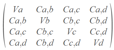
As you can see, the main diagonal is written as V (variance) and the rest is written as C (covariance), why is that?
Because calculating the covariance of the same variable is basically calculating its variance (if you’re not sure why — please take a few minutes to understand what variance and covariance are).
Let’s calculate in Python the covariance matrix of the dataset using the following code:
covarianceMatrix = pd.DataFrame(data = np.cov(dataset, rowvar = False), columns = irisModule.feature_names, index = irisModule.feature_names)
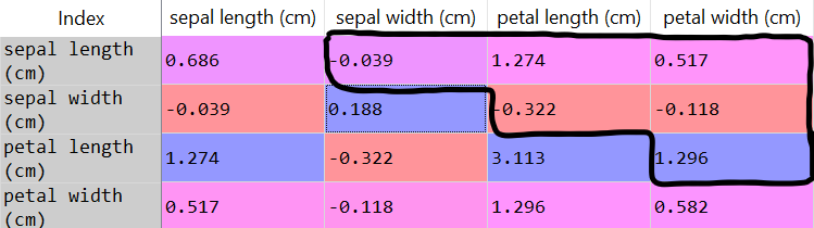
- We’re not interested in the main diagonal, because they are the variance of the same variable. Since we’re trying to find new patterns in the dataset, we’ll ignore the main diagonal.
- Since the matrix is symmetric, covariance(a,b) = covariance(b,a), we will look only at the top values of the covariance matrix (above diagonal).
Something important to mention about covariance: if the covariance of variables a and b is positive, that means they vary in the same direction. If the covariance of a and b is negative, they vary in different directions.
3) Calculate the eigenvalues and eigenvectors:
As I mentioned at the beginning, eigenvalues and eigenvectors are the basic terms you must know in order to understand this step. Therefore, I won’t explain it, but will rather move to compute them.
The eigenvector associated with the largest eigenvalue indicates the direction in which the data has the most variance. Hence, using eigenvalues we will know what eigenvectors capture the most variability in our data.
eigenvalues, eigenvectors = np.linalg.eig(covarianceMatrix)
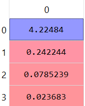
This is the vector of the eigenvalues, the first index at eigenvalues vector is associated with the first index at eigenvectors matrix.
The eigenvalues:
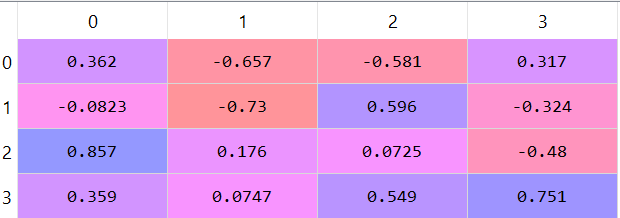
The eigenvectors matrix:
4) Choose the first K eigenvalues (K principal components/axises):
The eigenvalues tells us the amount of variability in the direction of its corresponding eigenvector. Therefore, the eigenvector with the largest eigenvalue is the direction with most variability. We call this eigenvector the first principle component (or axis). From this logic, the eigenvector with the second largest eigenvalue will be called the second principal component, and so on.
We see the following values:
[4.224, 0.242, 0.078, 0.023]
Let’s translate those values to percentages and visualize them. We’ll take the percentage that each eigenvalue covers in the dataset.
totalSum = sum(eigenvalues)variablesExplained = [(i / totalSum) for i in sorted(eigenvalues, reverse = True)]
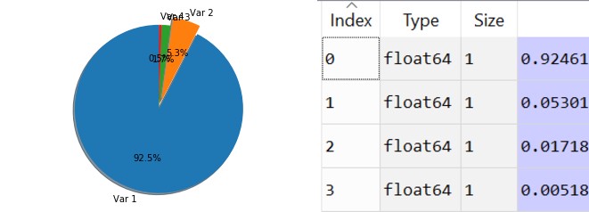
As you can clearly see the first and eigenvalue takes 92.5% and the second one takes 5.3%, and the third and forth don’t cover much data from the total dataset. Therefore we can easily decide to remain with only 2 variables, the first one and the second one.
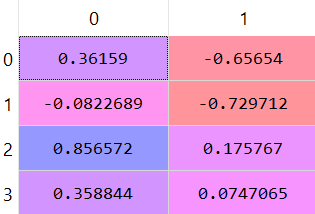
featureVector = eigenvectors[:,:2]
Let’s remove the third and fourth variables from the dataset. Important to say that at this point we lose some information. It is impossible to reduce dimensions without losing some information (under the assumption of general position). PCA algorithm tells us the right way to reduce dimensions while keeping the maximum amount of information regarding our data.
And the remaining data set looks like this:
5) Build the new reduced dataset:
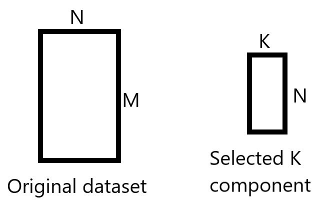
We want to build a new reduced dataset from the K chosen principle components.
We’ll take the K chosen principles component (k=2 here) which gives us a matrix of size (4, 2), and we will take the original dataset which is a matrix of size (150, 4).
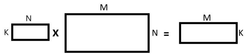
We’ll perform matrices multiplication in such a way:
- The first matrix we take is the matrix that contains the K component principles we’ve chosen and we transpose this matrix.
- The second matrix we take is the original matrix and we transpose it.
- At this point, we perform matrix multiplication between those two matrices.
- After we perform matrix multiplication we transpose the result matrix.
featureVectorTranspose = np.transpose(featureVector)datasetTranspose = np.transpose(dataset)newDatasetTranspose = np.matmul(featureVectorTranspose, datasetTranspose)newDataset = np.transpose(newDatasetTranspose)
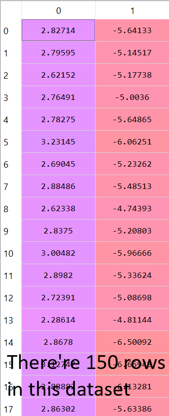
After performing the matrices multiplication and transposing the result matrix, these are the values we get for the new data which contains only the K principal components we’ve chosen.
Conclusion
As (we hope) you can now see, PCA is not that hard. We’ve managed to reduce the dimensions of the dataset pretty easily using Python.
In our data set, we did not cause serious impact because we removed only 2 variables out of 4. But let’s assume we have 200 variables in our data set, and we reduced from 200 variables to 3 variables — it’s already becoming more meaningful.
Hopefully, you’ve learned something new today. Feel free to contact Chen Shani or Moshe Binieli on Linkedin for any questions.