

Do you really understand Big O? If so, then this will refresh your understanding before an interview. If not, don’t worry — come and join us for some endeavors in computer science.
If you have taken some algorithm related courses, you’ve probably heard of the term Big O notation. If you haven’t, we will go over it here, and then get a deeper understanding of what it really is.
Big O notation is one of the most fundamental tools for computer scientists to analyze the cost of an algorithm. It is a good practice for software engineers to understand in-depth as well.
This article is written with the assumption that you have already tackled some code. Also, some in-depth material also requires high-school math fundamentals, and therefore can be a bit less comfortable to total beginners. But if you are ready, let’s get started!
In this article, we will have an in-depth discussion about Big O notation. We will start with an example algorithm to open up our understanding. Then, we will go into the mathematics a little bit to have a formal understanding. After that we will go over some common variations of Big O notation. In the end, we will discuss some of the limitations of Big O in a practical scenario. A table of contents can be found below.
Table of Contents
- What is Big O notation, and why does it matter
- Formal Definition of Big O notation
- Big O, Little O, Omega & Theta
- Complexity Comparison Between Typical Big Os
- Time & Space Complexity
- Best, Average, Worst, Expected Complexity
- Why Big O doesn’t matter
- In the end…
So let’s get started.
1. What is Big O Notation, and why does it matter
“Big O notation is a mathematical notation that describes the limiting behavior of a function when the argument tends towards a particular value or infinity. It is a member of a family of notations invented by Paul Bachmann, Edmund Landau, and others, collectively called Bachmann–Landau notation or asymptotic notation.”
— Wikipedia’s definition of Big O notation
In plain words, Big O notation describes the complexity of your code using algebraic terms.
To understand what Big O notation is, we can take a look at a typical example, O(n²), which is usually pronounced “Big O squared”. The letter “n” here represents the input size, and the function “g(n) = n²” inside the “O()” gives us an idea of how complex the algorithm is with respect to the input size.
A typical algorithm that has the complexity of O(n²) would be the selection sort algorithm. Selection sort is a sorting algorithm that iterates through the list to ensure every element at index i is the ith smallest/largest element of the list. The CODEPEN below gives a visual example of it.
The algorithm can be described by the following code. In order to make sure the ith element is the ith smallest element in the list, this algorithm first iterates through the list with a for loop. Then for every element it uses another for loop to find the smallest element in the remaining part of the list.
SelectionSort(List) {
  for(i from 0 to List.Length) {
    SmallestElement = List[i]
    for(j from i to List.Length) {
      if(SmallestElement > List[j]) {
        SmallestElement = List[j]
      }
    }
    Swap(List[i], SmallestElement)
  }
}
In this scenario, we consider the variable List as the input, thus input size n is the number of elements inside List. Assume the if statement, and the value assignment bounded by the if statement, takes constant time. Then we can find the big O notation for the SelectionSort function by analyzing how many times the statements are executed.
First the inner for loop runs the statements inside n times. And then after i is incremented, the inner for loop runs for n-1 times… …until it runs once, then both of the for loops reach their terminating conditions.
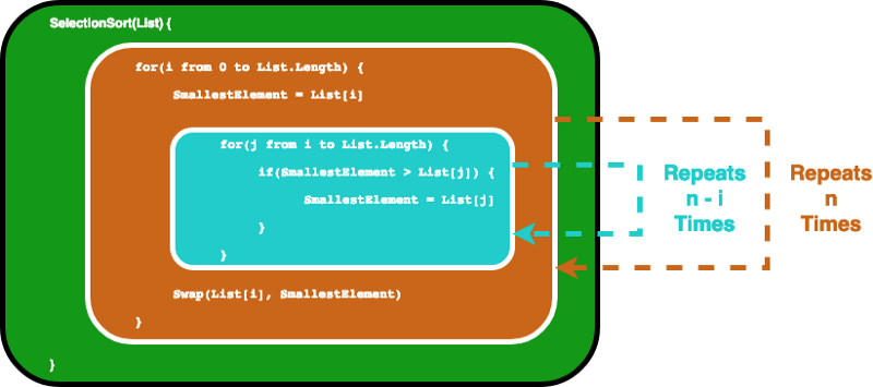
This actually ends up giving us a geometric sum, and with some high-school math we would find that the inner loop will repeat for 1+2 … + n times, which equals n(n-1)/2 times. If we multiply this out, we will end up getting n²/2-n/2.
When we calculate big O notation, we only care about the dominant terms, and we do not care about the coefficients. Thus we take the n² as our final big O. We write it as O(n²), which again is pronounced “Big O squared”.
Now you may be wondering, what is this “dominant term” all about? And why do we not care about the coefficients? Don’t worry, we will go over them one by one. It may be a little bit hard to understand at the beginning, but it will all make a lot more sense as you read through the next section.
2. Formal Definition of Big O notation
Once upon a time there was an Indian king who wanted to reward a wise man for his excellence. The wise man asked for nothing but some wheat that would fill up a chess board.
But here were his rules: in the first tile he wants 1 grain of wheat, then 2 on the second tile, then 4 on the next one…each tile on the chess board needed to be filled by double the amount of grains as the previous one. The naïve king agreed without hesitation, thinking it would be a trivial demand to fulfill, until he actually went on and tried it…
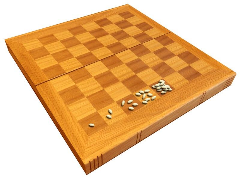
So how many grains of wheat does the king owe the wise man? We know that a chess board has 8 squares by 8 squares, which totals 64 tiles. So the last tile should have a total of 2⁶³ grains of wheat. If you do a calculation online, for the entire chessboard, you will end up getting 1.8446744*10¹⁹ – that is about 18 followed by 18 zeroes.
Assuming that each grain of wheat weights 0.01 grams, that gives us 184,467,440,737 tons of wheat. And 184 billion tons is quite a lot, isn’t it?
The numbers grow quite fast later for exponential growth don’t they? The same logic goes for computer algorithms. If the required efforts to accomplish a task grow exponentially with respect to the input size, it can end up becoming enormously large.
As we will see in a moment, the growth of 2ⁿ is much faster than n². Now, with n = 64, the square of 64 is 4096. If you add that number to 2⁶⁴, it will be lost outside the significant digits.
This is why, when we look at the growth rate, we only care about the dominant terms. And since we want to analyze the growth with respect to the input size, the coefficients which only multiply the number rather than growing with the input size do not contain useful information.
Below is the formal definition of Big O:

The formal definition is useful when you need to perform a math proof. For example, the time complexity for selection sort can be defined by the function f(n) = n²/2-n/2 as we have discussed in the previous section.
If we allow our function g(n) to be n², we can find a constant c = 1, and a N₀ = 0, and so long as N > N₀, N² will always be greater than N²/2-N/2. We can easily prove this by subtracting N²/2 from both functions, then we can easily see N²/2 > -N/2 to be true when N > 0. Therefore, we can come up with the conclusion that f(n) = O(n²), in the other selection sort is “big O squared”.
You might have noticed a little trick here. That is, if you make g(n) grow super fast, way faster than anything, O(g(n)) will always be great enough. For example, for any polynomial function, you can always be right by saying that they are O(2ⁿ) because 2ⁿ will eventually outgrow any polynomials.
Mathematically, you are right, but generally when we talk about Big O, we want to know the tight bound of the function. You will understand this more as you read through the next section.
But before we go, let’s test your understanding with the following question. The answer will be found in later sections so it won’t be a throw away.
Question: An image is represented by a 2D array of pixels. If you use a nested for loop to iterate through every pixel (that is, you have a for loop going through all the columns, then another for loop inside to go through all the rows), what is the time complexity of the algorithm when the image is considered as the input?
3. Big O, Little O, Omega & Theta
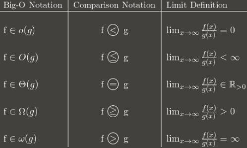
Big O: “f(n) is O(g(n))” iff for some constants c and N₀, f(N) ≤ cg(N) for all N > N₀
Omega: “f(n) is Ω(g(n))” iff for some constants c and N₀, f(N) ≥ cg(N) for all N > N₀
Theta: “f(n) is Θ(g(n))” iff f(n) is O(g(n)) and f(n) is Ω(g(n))
Little O: “f(n) is o(g(n))” iff f(n) is O(g(n)) and f(n) is not Θ(g(n))
—Formal Definition of Big O, Omega, Theta and Little O
In plain words:
- Big O (O()) describes the upper bound of the complexity.
- Omega (Ω()) describes the lower bound of the complexity.
- Theta (Θ()) describes the exact bound of the complexity.
- Little O (o()) describes the upper bound excluding the exact bound.
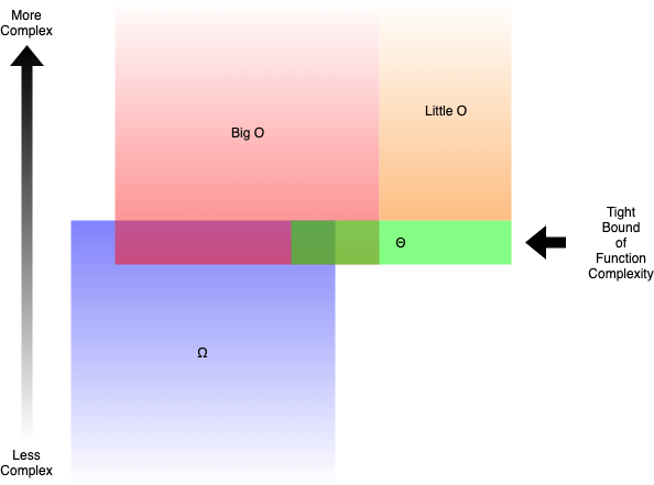
For example, the function g(n) = n² + 3n is O(n³), o(n⁴), Θ(n²) and Ω(n). But you would still be right if you say it is Ω(n²) or O(n²).
Generally, when we talk about Big O, what we actually meant is Theta. It is kind of meaningless when you give an upper bound that is way larger than the scope of the analysis. This would be similar to solving inequalities by putting ∞ on the larger side, which will almost always make you right.
But how do we determine which functions are more complex than others? In the next section you will be reading, we will learn that in detail.
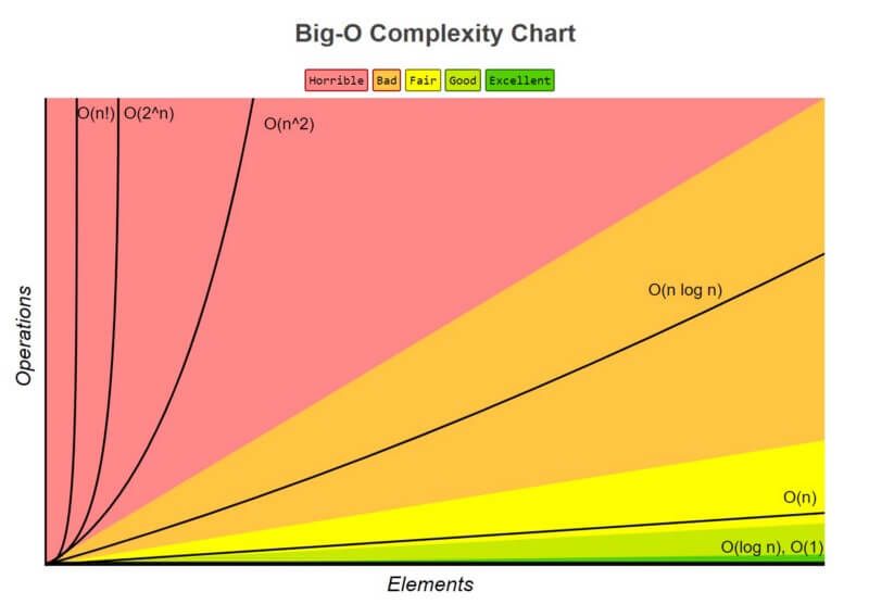
4. Complexity Comparison Between Typical Big Os
When we are trying to figure out the Big O for a particular function g(n), we only care about the dominant term of the function. The dominant term is the term that grows the fastest.
For example, n² grows faster than n, so if we have something like g(n) = n² + 5n + 6, it will be big O(n²). If you have taken some calculus before, this is very similar to the shortcut of finding limits for fractional polynomials, where you only care about the dominant term for numerators and denominators in the end.
But which function grows faster than the others? There are actually quite a few rules.
1. O(1) has the least complexity
Often called “constant time”, if you can create an algorithm to solve the problem in O(1), you are probably at your best. In some scenarios, the complexity may go beyond O(1), then we can analyze them by finding its O(1/g(n)) counterpart. For example, O(1/n) is more complex than O(1/n²).
2. O(log(n)) is more complex than O(1), but less complex than polynomials
As complexity is often related to divide and conquer algorithms, O(log(n)) is generally a good complexity you can reach for sorting algorithms. O(log(n)) is less complex than O(√n), because the square root function can be considered a polynomial, where the exponent is 0.5.
3. Complexity of polynomials increases as the exponent increases
For example, O(n⁵) is more complex than O(n⁴). Due to the simplicity of it, we actually went over quite many examples of polynomials in the previous sections.
4. Exponentials have greater complexity than polynomials as long as the coefficients are positive multiples of n
O(2ⁿ) is more complex than O(n⁹⁹), but O(2ⁿ) is actually less complex than O(1). We generally take 2 as base for exponentials and logarithms because things tends to be binary in Computer Science, but exponents can be changed by changing the coefficients. If not specified, the base for logarithms is assumed to be 2.
5. Factorials have greater complexity than exponentials
If you are interested in the reasoning, look up the Gamma function, it is an analytic continuation of a factorial. A short proof is that both factorials and exponentials have the same number of multiplications, but the numbers that get multiplied grow for factorials, while remaining constant for exponentials.
6. Multiplying terms
When multiplying, the complexity will be greater than the original, but no more than the equivalence of multiplying something that is more complex. For example, O(n * log(n)) is more complex than O(n) but less complex than O(n²), because O(n²) = O(n * n) and n is more complex than log(n).
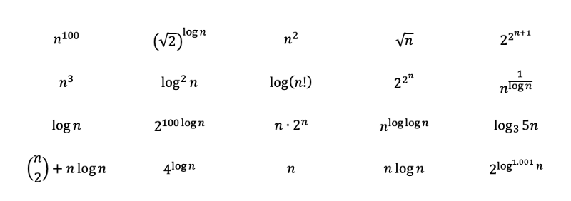
To test your understanding, try ranking the following functions from the most complex to the least complex. The solutions with detailed explanations can be found in a later section as you read. Some of them are meant to be tricky and may require some deeper understanding of math. As you get to the solution, you will understand them more.
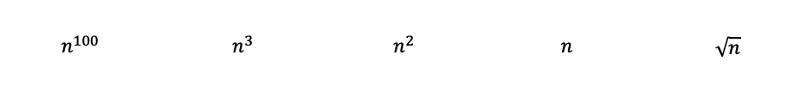
Question: Rank following functions from the most complex to the least complex.
Solution to Section 2 Question:
It was actually meant to be a trick question to test your understanding. The question tries to make you answer O(n²) because there is a nested for loop. However, n is supposed to be the input size. Since the image array is the input, and every pixel was iterated through only once, the answer is actually O(n). The next section will go over more examples like this one.
5. Time & Space Complexity
So far, we have only been discussing the time complexity of the algorithms. That is, we only care about how much time it takes for the program to complete the task. What also matters is the space the program takes to complete the task. The space complexity is related to how much memory the program will use, and therefore is also an important factor to analyze.
The space complexity works similarly to time complexity. For example, selection sort has a space complexity of O(1), because it only stores one minimum value and its index for comparison, the maximum space used does not increase with the input size.
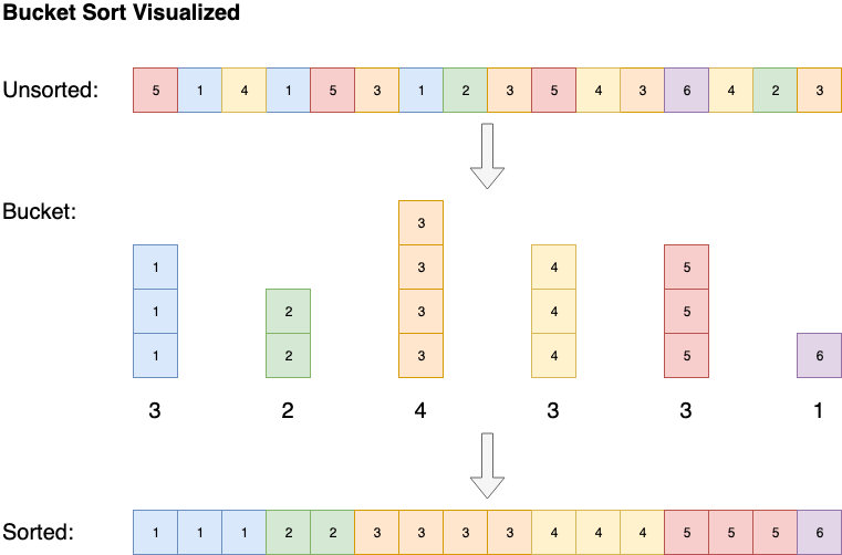
Some algorithms, such as bucket sort, have a space complexity of O(n), but are able to chop down the time complexity to O(1). Bucket sort sorts the array by creating a sorted list of all the possible elements in the array, then increments the count whenever the element is encountered. In the end the sorted array will be the sorted list elements repeated by their counts.
6. Best, Average, Worst, Expected Complexity
The complexity can also be analyzed as best case, worst case, average case and expected case.
Let’s take insertion sort, for example. Insertion sort iterates through all the elements in the list. If the element is smaller than its previous element, it inserts the element backwards until it is larger than the previous element.
If the array is initially sorted, no swap will be made. The algorithm will just iterate through the array once, which results a time complexity of O(n). Therefore, we would say that the best-case time complexity of insertion sort is O(n). A complexity of O(n) is also often called linear complexity.
Sometimes an algorithm just has bad luck. Quick sort, for example, will have to go through the list in O(n) time if the elements are sorted in the opposite order, but on average it sorts the array in O(n * log(n)) time. Generally, when we evaluate time complexity of an algorithm, we look at their worst-case performance. More on that and quick sort will be discussed in the next section as you read.
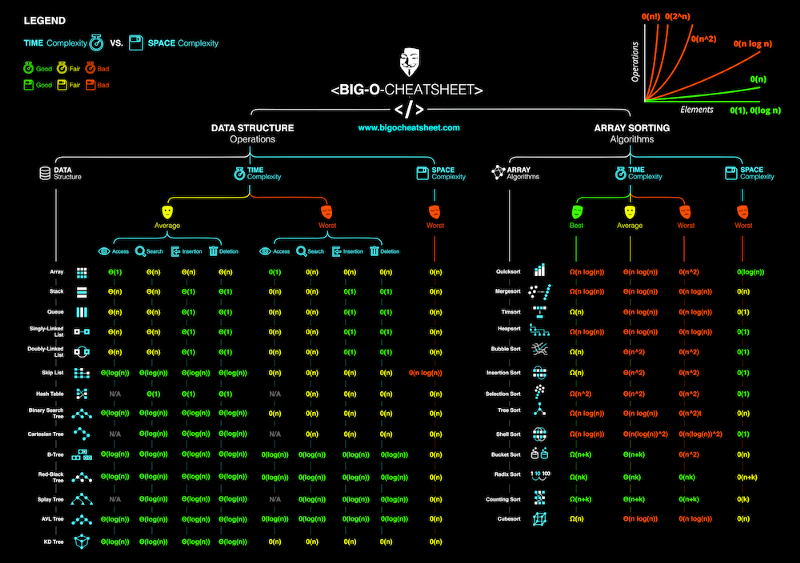
The average case complexity describes the expected performance of the algorithm. Sometimes involves calculating the probability of each scenarios. It can get complicated to go into the details and therefore not discussed in this article. Below is a cheat-sheet on the time and space complexity of typical algorithms.
Solution to Section 4 Question:
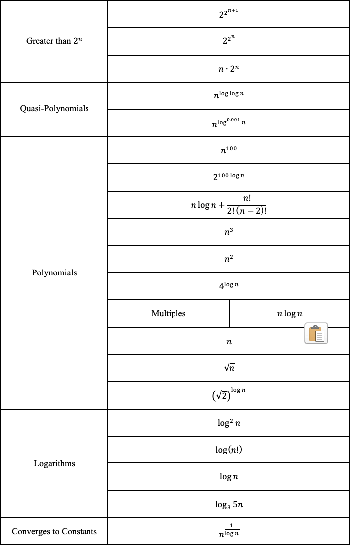
By inspecting the functions, we should be able to immediately rank the following polynomials from most complex to least complex with rule 3. Where the square root of n is just n to the power of 0.5.
Then by applying rules 2 and 6, we will get the following. Base 3 log can be converted to base 2 with log base conversions. Base 3 log still grows a little bit slower then base 2 logs, and therefore gets ranked after.

The rest may look a little bit tricky, but let’s try to unveil their true faces and see where we can put them.
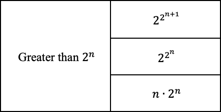
First of all, 2 to the power of 2 to the power of n is greater than 2 to the power of n, and the +1 spices it up even more.
And then since we know 2 to the power of log(n) with based 2 is equal to n, we can convert the following. The log with 0.001 as exponent grows a little bit more than constants, but less than almost anything else.
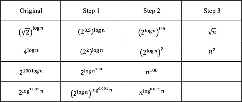
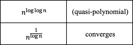
The one with n to the power of log(log(n)) is actually a variation of the quasi-polynomial, which is greater than polynomial but less than exponential. Since log(n) grows slower than n, the complexity of it is a bit less. The one with the inverse log converges to constant, as 1/log(n) diverges to infinity.
The factorials can be represented by multiplications, and thus can be converted to additions outside the logarithmic function. The “n choose 2” can be converted into a polynomial with a cubic term being the largest.
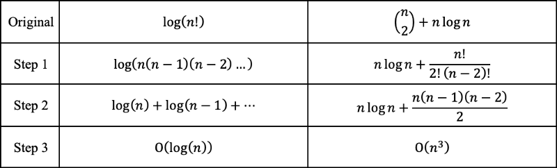
And finally, we can rank the functions from the most complex to the least complex.
Why BigO doesn’t matter
!!! — WARNING — !!!
Contents discussed here are generally not accepted by most programmers in the world. Discuss it at your own risk in an interview. People actually blogged about how they failed their Google interviews because they questioned the authority, like here.
!!! — WARNING — !!!
Since we have previously learned that the worst case time complexity for quick sort is O(n²), but O(n * log(n)) for merge sort, merge sort should be faster — right? Well you probably have guessed that the answer is false. The algorithms are just wired up in a way that makes quick sort the “quick sort”.
To demonstrate, check out this trinket.io I made. It compares the time for quick sort and merge sort. I have only managed to test it on arrays with a length up to 10000, but as you can see so far, the time for merge sort grows faster than quick sort. Despite quick sort having a worse case complexity of O(n²), the likelihood of that is really low. When it comes to the increase in speed quick sort has over merge sort bounded by the O(n * log(n)) complexity, quick sort ends up with a better performance in average.
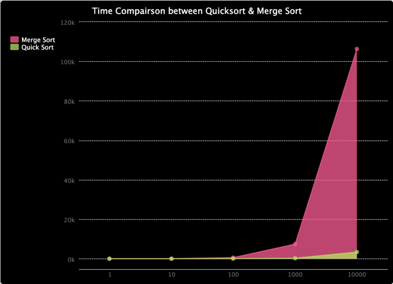
I have also made the below graph to compare the ratio between the time they take, as it is hard to see them at lower values. And as you can see, the percentage time taken for quick sort is in a descending order.
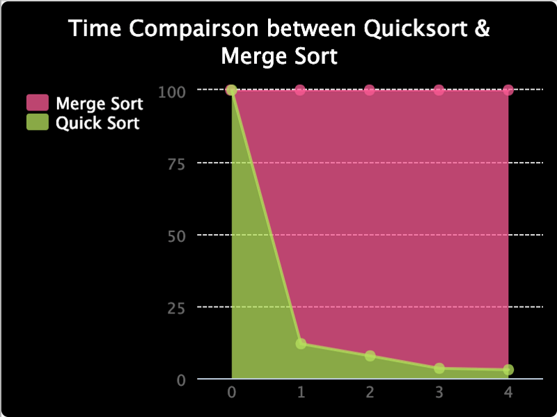
The moral of the story is, Big O notation is only a mathematical analysis to provide a reference on the resources consumed by the algorithm. Practically, the results may be different. But it is generally a good practice trying to chop down the complexity of our algorithms, until we run into a case where we know what we are doing.
In the end…
I like coding, learning new things and sharing them with the community. If there is anything in which you are particularly interested, please let me know. I generally write on web design, software architecture, mathematics and data science. You can find some great articles I have written before if you are interested in any of the topics above.
Hope you have a great time learning computer science!!!