
Binary classification is a fundamental task in machine learning, where the goal is to categorize data into one of two classes or categories.
Binary classification is used in a wide range of applications, such as spam email detection, medical diagnosis, sentiment analysis, fraud detection, and many more.
In this article, we'll explore binary classification using TensorFlow, one of the most popular deep learning libraries.
Before getting into the Binary Classification, let's discuss a little about classification problem in Machine Learning.
What is Classification problem?
A Classification problem is a type of machine learning or statistical problem in which the goal is to assign a category or label to a set of input data based on their characteristics or features. The objective is to learn a mapping between input data and predefined classes or categories, and then use this mapping to predict the class labels of new, unseen data points.
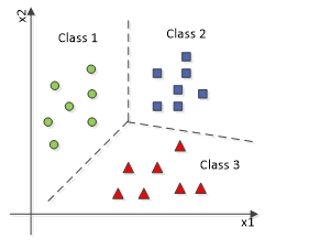 Sample Multi Classification
The above diagram represents a multi-classification problem in which the data will be classified into more than two (three here) types of classes.
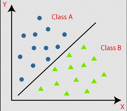 Sample Binary Classification
This diagram defines Binary Classification, where data is classified into two type of classes.
This simple concept is enough to understand classification problems. Let's explore this with a real-life example.
Heart Attack Analytics Prediction Using Binary Classification
In this article, we will embark on the journey of constructing a predictive model for heart attack analysis utilizing straightforward deep learning libraries.
The model that we'll be building, while being a relatively simple neural network, is capable of achieving an accuracy level of approximately 80%.
Solving real-world problems through the lens of machine learning entails a series of essential steps:
- Data Collection and Analytics
- Data preprocessing
- Building ML Model
- Train the Model
- Prediction and Evaluation
Data Collection and Analytics
It's worth noting that for this project, I obtained the dataset from Kaggle, a popular platform for data science competitions and datasets.
I encourage you to take a closer look at its contents. Understanding the dataset is crucial as it allows you to grasp the nuances and intricacies of the data, which can help you make informed decisions throughout the machine learning pipeline.
This dataset is well-structured, and there's no immediate need for further analysis. However, if you are collecting the dataset on your own, you will need to perform data analytics and visualization independently to achieve better accuracy.
Let's put on our coding shoes.
Here I am using Google Colab. You can use your own machine (in which case you will need to create a .ipynb file) or Google Colab on your account to run the notebook. You can find my source code here.
As the first step, let's import the required libraries.
import numpy as np
import matplotlib.pyplot as plt
from sklearn.model_selection import train_test_split
import sklearn
import pandas as pd
import keras
from keras.models import Sequential
from keras.layers import Dense
import tensorflow as tf
from sklearn.metrics import confusion_matrix,ConfusionMatrixDisplay
from sklearn.preprocessing import MinMaxScaler
I have the dataset in my drive and I'm reading it from my drive. You can download the same dataset here.
Remember the replace the path of your file in the read_csv method:
df = pd.read_csv("/content/drive/MyDrive/Datasets/heart.csv")
df.head()
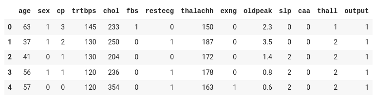 Sample 5 record in the dataset
The dataset contains thirteen input columns (age, sex, cp, and so on) and one output column (output), which will contain the data as either 0 or 1.
Considering the input readings, 0 in the output represents the person will not get heart attack, while the 1 represents the person will be affected by heart attack.
Let's split our input and output from the above dataset to train our model:
target_column = "output"
numerical_column = df.columns.drop(target_column)
output_rows = df[target_column]
df.drop(target_column,axis=1,inplace=True)
Since our objective is to predict the likelihood of a heart attack (0 or 1), represented by the target column, we split that into a separate dataset.
Data preprocessing
Data preprocessing is a crucial step in the machine learning pipeline, and binary classification is no exception. It involves the cleaning, transformation, and organization of raw data into a format that is suitable for training machine learning models.
A dataset will contain multiple type of data such as Numerical Data, Categorical Data, Timestamp Data, and so on.
But most of the Machine Learning algorithms are designed to work with numerical data. They require input data to be in a numeric format for mathematical operations, optimization, and model training.
In this dataset, all the columns contain numerical data, so we don't need to encode the data. We can proceed with simple normalization.
Remember if you have any non-numerical columns in your dataset, you may have to convert it into numerical by performing one-hot encoding or using other encoding algorithms.
There are lot of normalization strategies. Here I am using Min-Max Normalization:
 Min-Max Scaling Formula
Don't worry – we don't need to apply this formula manually. We have some machine learning libraries to do this. Here I am using MinMaxScaler from sklearn:
scaler = MinMaxScaler()
scaler.fit(df)
t_df = scaler.transform(df)
scaler.fit(df) computes the mean and standard deviation (or other scaling parameters) necessary to perform the scaling operation. The fit method essentially learns these parameters from the data.
t_df = scaler.transform(df): After fitting the scaler, we need to transform the dataset. The transformation typically scales the features to have a mean of 0 and a standard deviation of 1 (standardization) or scales them to a specific range (for example, [0, 1] with Min-Max scaling) depending on the scaler used.
We have completed the preprocessing. The next crucial step is to split the dataset into training and testing sets.
To accomplish this, I will utilize the train_test_split function from scikit-learn.
X_train and X_test are the variables that hold the independent variables.
y_train and y_test are the variables that hold the dependent variable, which represents the output we are aiming to predict.
X_train, X_test, y_train, y_test = train_test_split(t_df, output_rows, test_size=0.25, random_state=0)
print('X_train:',np.shape(X_train))
print('y_train:',np.shape(y_train))
print('X_test:',np.shape(X_test))
print('y_test:',np.shape(y_test))
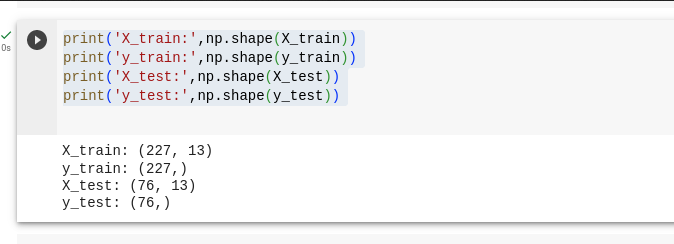 Sample training and testing dataset size
We split the dataset by 75% and 25%, where 75% goes for training our model and 25% goes for testing our model.
Building ML Model
A machine learning model is a computational representation of a problem or a system that is designed to learn patterns, relationships, and associations from data. It serves as a mathematical and algorithmic framework capable of making predictions, classifications, or decisions based on input data.
In essence, a model encapsulates the knowledge extracted from data, allowing it to generalize and make informed responses to new, previously unseen data.
Here, I am building a simple sequential model with one input layer and one output layer. Being a simple model, I am not using any hidden layer as it might increase the complexity of the concept.
Initialize Sequential Model
basic_model = Sequential()
Sequential is a type of model in Keras that allows you to create neural networks layer by layer in a sequential manner. Each layer is added on top of the previous one.
Input Layer
basic_model.add(Dense(units=16, activation='relu', input_shape=(13,)))
Dense is a type of layer in Keras, representing a fully connected layer. It has 16 units, which means it has 16 neurons.
activation='relu' specifies the Rectified Linear Unit (ReLU) activation function, which is commonly used in input or hidden layers of neural networks.
input_shape=(13,) indicates the shape of the input data for this layer. In this case, we are using 13 input features (columns).
Output Layer
basic_model.add(Dense(1, activation='sigmoid'))
This line adds the output layer to the model.
It's a single neuron (1 unit) because this appears to be a binary classification problem, where you're predicting one of two classes (0 or 1).
The activation function used here is 'sigmoid', which is commonly used for binary classification tasks. It squashes the output to a range between 0 and 1, representing the probability of belonging to one of the classes.
Optimizer
adam = keras.optimizers.Adam(learning_rate=0.001)
This line initializes the Adam optimizer with a learning rate of 0.001. The optimizer is responsible for updating the model's weights during training to minimize the defined loss function.
Compile Model
basic_model.compile(loss='binary_crossentropy', optimizer=adam, metrics=["accuracy"])
Here, we'll compile the model.
loss='binary_crossentropy' is the loss function used for binary classification. It measures the difference between the predicted and actual values and is minimized during training.
metrics=["accuracy"]: During training, we want to monitor the accuracy metric, which tells you how well the model is performing in terms of correct predictions.
Train model with dataset
Hurray, we built the model. Now it's time to train the model with our training dataset.
basic_model.fit(X_train, y_train, epochs=100)
X_train represents the training data, which consists of the independent variables (features). The model will learn from these features to make predictions or classifications.
y_train are the corresponding target labels or dependent variables for the training data. The model will use this information to learn the patterns and relationships between the features and the target variable.
epochs=100: The epochs parameter specifies the number of times the model will iterate over the entire training dataset. Each pass through in the dataset is called an epoch. In this case, we have 100 epochs, meaning the model will see the entire training dataset 100 times during training.
loss_and_metrics = basic_model.evaluate(X_test, y_test)
print(loss_and_metrics)
print('Loss = ',loss_and_metrics[0])
print('Accuracy = ',loss_and_metrics[1])
The evaluate method is used to assess how well the trained model performs on the test dataset. It computes the loss (often the same loss function used during training) and any specified metrics (for example, accuracy) for the model's predictions on the test data.
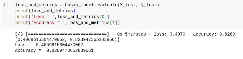 Sample output to find the Loss and Accuracy
Here we got around 82% accuracy.
Prediction and Evaluation
predicted = basic_model.predict(X_test)
The predict method is used to generate predictions from the model based on the input data (X_test in this case). The output (predicted) will contain the model's predictions for each data point in the training dataset.
Since I have only minimum dataset I am using the test dataset for prediction. However, it is a recommend practice to split a part of dataset (say 10%) to use as a validation dataset.
Evaluation
Evaluating predictions in machine learning is a crucial step to assess the performance of a model.
One commonly tool used for evaluating classification models is the confusion matrix. Let's explore what a confusion matrix is and how it's used for model evaluation:
In a binary classification problem (two classes, for example, "positive" and "negative"), a confusion matrix typically looks like this:
| Predicted Negative (0) | Predicted Positive (1) | |
| Actual Negative (0) | True Negative | False Positive |
| Actual Positive (1) | False Negative | True Positive |
Here's the code to plot the confusion matrix from the predicted data of our model:
predicted = tf.squeeze(predicted)
predicted = np.array([1 if x >= 0.5 else 0 for x in predicted])
actual = np.array(y_test)
conf_mat = confusion_matrix(actual, predicted)
displ = ConfusionMatrixDisplay(confusion_matrix=conf_mat)
displ.plot()
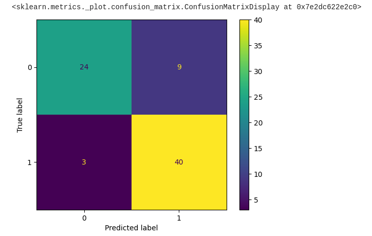 Confusion matrix for the predicted output
Bravo! We've made significant progress toward obtaining the required output, with approximately 84% of the data appearing to be correct.
It's worth noting that we can further optimize this model by leveraging a larger dataset and fine-tuning the hyper-parameters. However, for a foundational understanding, what we've accomplished so far is quite impressive.
Given that this dataset and the corresponding machine learning models are at a very basic level, it's important to acknowledge that real-world scenarios often involve much more complex datasets and machine learning tasks.
While this model may perform adequately for simple problems, it may not be suitable for tackling more intricate challenges.
In real-world applications, datasets can be vast and diverse, containing a multitude of features, intricate relationships, and hidden patterns. Consequently, addressing such complexities often demands a more sophisticated approach.
Here are some key factors to consider when working with complex datasets.
- Complex Data Preprocessing
- Advanced Data Encoding
- Understanding Data Correlation
- Multiple Neural Network Layers
- Feature Engineering
- Regularization
If you're already familiar with building a basic neural network, I highly recommend delving into these concepts to excel in the world of Machine Learning.
Conclusion
In this article, we embarked on a journey into the fascinating world of machine learning, starting with the basics.
We explored the fundamentals of binary classification—a fundamental machine learning task. From understanding the problem to building a simple model, we've gained insights into the foundational concepts that underpin this powerful field.
So, whether you're just starting or already well along the path, keep exploring, experimenting, and pushing the boundaries of what's possible with machine learning. I'll see you in another exciting article!
If you wish to learn more about artificial intelligence / machine learning / deep learning, subscribe to my article by visiting my site, which has a consolidated list of all my articles.