
By Aditya
Image classification is an amazing application of deep learning. We can train a powerful algorithm to model a large image dataset. This model can then be used to classify a similar but unknown set of images.
There is no limit to the applications of image classification. You can use it in your next app or you can use it to solve some real world problem. That's all up to you. But to someone who is fairly new to this realm, it might seem very challenging at first. How should I get my data? How should I build my model? What tools should I use?
In this article we will discuss all of that - from finding a dataset to training your model. I will try to make things as simple as possible by avoiding some technical details (PS: Please note that this doesn't mean those details are not important. I will mention some great resources which you can refer to learn more about those topics). The purpose of this article is to explain the basic process of building an image classifier and that's what we will focus more on here.
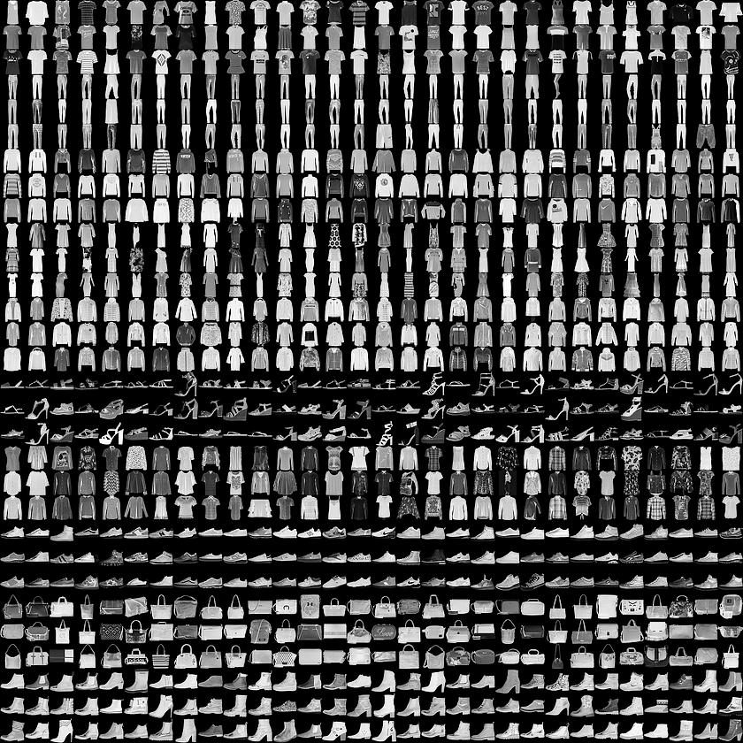
We will build an Image classifier for the Fashion-MNIST Dataset. The Fashion-MNIST dataset is a collection of Zalando's article images. It contains 60,000 images for the training set and 10,000 images for the test set data (we will discuss the test and training datasets along with the validation dataset later). These images belong to the labels of 10 different classes.
Importing Libraries
Our goal is to train a deep learning model that can classify a given set of images into one of these 10 classes. Now that we have our dataset, we should move on to the tools we need. There are many libraries and tools out there that you can choose based on your own project requirements. For this one I will stick to the following:
- Numpy - Python library for numerical computation
- Pandas - Python library data manipulation
- Matplotlib - Python library data visualisation
- Keras - Python library based on tensorflow for creating deep learning models
- Jupyter - I will run all my code on Jupyter Notebooks. You can install it via the link. You can use Google Colabs also if you need better computational power.
Along with these four, we will also use scikit-learn. The purpose of these libraries will become more clear once we dive into the code.
Okay! We have our tools and libraries ready. Now we should start setting up our code.
Start with importing all the above mentioned libraries. Along with importing libraries I have also imported some specific modules from these libraries. Let me go through them one by one.
import numpy as np
import pandas as pd
import matplotlib.pyplot as plt
import keras

from sklearn.model_selection import train_test_split
from keras.utils import to_categorical

from keras.models import Sequential
from keras.layers import Conv2D, MaxPooling2D
from keras.layers import Dense, Dropout
from keras.layers import Flatten, BatchNormalization
train_test_split: This module splits the training dataset into training and validation data. The reason behind this split is to check if our model is overfitting or not. We use a training dataset to train our model and then we will compare the resulting accuracy to validation accuracy. If the difference between both quantities is significantly large, then our model is probably overfitting. We will reiterate through our model building process and making required changes along the way. Once we are satisfied with our training and validation accuracies, we will make final predictions on our test data.
to_categorical: to_categorical is a keras utility. It is used to convert the categorical labels into one-hot encodings. Let's say we have three labels ("apples", "oranges", "bananas"), then one hot encodings for each of these would be [1, 0, 0] -> "apples", [0, 1, 0] -> "oranges", [0, 0, 1] -> "bananas".
The rest of the Keras modules we have imported are convolutional layers. We will discuss convolutional layers when we start building our model. We will also give a quick glance to what each of these layers do.
Data Pre-processing
For now we will shift our attention to getting our data and analysing it. You should always remember the importance of pre-processing and analysing the data. It not only gives you insights about the data but also helps to locate inconsistencies.
A very slight variation in data can sometimes lead to a devastating result for your model. This makes it important to preprocess your data before using it for training. So with that in mind let's start data preprocessing.
train_df = pd.read_csv('./fashion-mnist_train.csv')
test_df = pd.read_csv('./fashion-mnist_test.csv')
First of all let's import our dataset (Here is the link to download this dataset on your system). Once you have imported the dataset, run the following command.
train_df.head()
This command will show you how your data looks like. The following screenshot shows the output of this command.
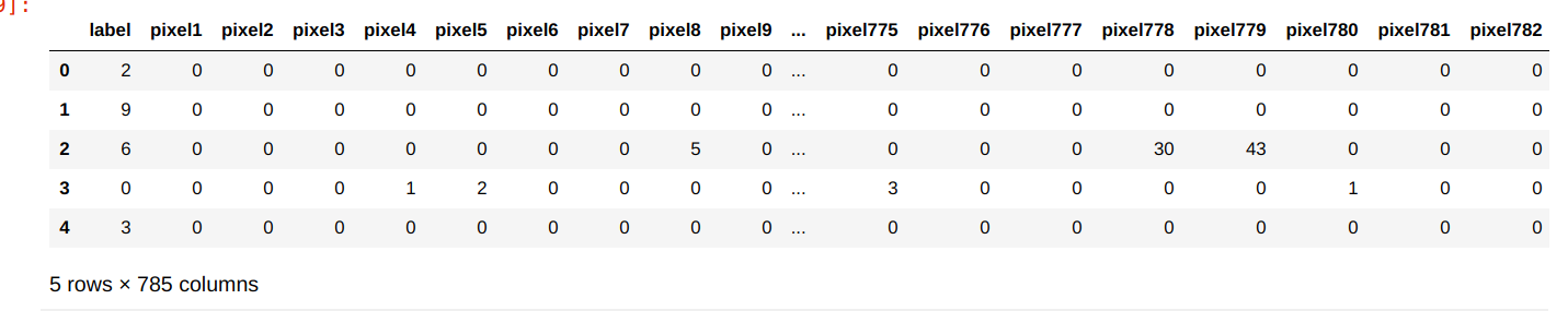
We can see how our image data is stored in the form of pixel values. But we cannot feed data to our model in this format. So, we will have to convert it into numpy arrays.
train_data = np.array(train_df.iloc[:, 1:])
test_data = np.array(test_df.iloc[:, 1:])
Now, it's time to get our labels.
train_labels = to_categorical(train_df.iloc[:, 0])
test_labels = to_categorical(test_df.iloc[:, 0])
Here, you can see that we have used _tocategorical to convert our categorical data into one hot encodings.
We will now reshape the data and cast it into float32 type so that we can use it conveniently.
rows, cols = 28, 28

train_data = train_data.reshape(train_data.shape[0], rows, cols, 1)
test_data = test_data.reshape(test_data.shape[0], rows, cols, 1)

train_data = train_data.astype('float32')
test_data = test_data.astype('float32')
We are almost done. Let's just finish preprocessing our data by normalizing it. Normalizing image data will map all the pixel values in each image to the values between 0 to 1. This helps us reduce inconsistencies in data. Before normalizing, the image data can have large variations in pixel values which can lead to some unusual behaviour during the training process.
train_data /= 255.0
test_data /= 255.0
Convolutional Neural Networks
So, data preprocessing is done. Now we can start building our model. We will build a Convolutional Neural Network for modeling the image data. CNNs are modified versions of regular neural networks. These are modified specifically for image data. Feeding images to regular neural networks would require our network to have a large number of input neurons. For example just for a 28x28 image we would require 784 input neurons. This would create a huge mess of training parameters.
CNNs fix this problem by already assuming that the input is going to be an image. The main purpose of convolutional neural networks is to take advantage of the spatial structure of the image and to extract high level features from that and then train on those features. It does so by performing a convolution operation on the matrix of pixel values.
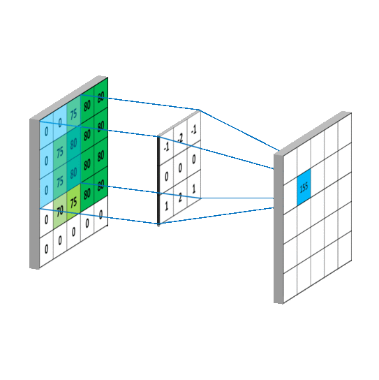
The visualization above shows how convolution operation works. And the Conv2D layer we imported earlier does the same thing. The first matrix (from the left) in the demonstration is the input to the convolutional layer. Then another matrix called "filter" or "kernel" is multiplied (matrix multiplication) to each window of the input matrix. The output of this multiplication is the input to the next layer.
Other than convolutional layers, a typical CNN also has two other types of layers: 1) a pooling layer, and 2) a fully connected layer.
Pooling layers are used to generalize the output of the convolutional layers. Along with generalizing, it also reduces the number of parameters in the model by down-sampling the output of the convolutional layer.
As we just learned, convolutional layers represent high level features from image data. Fully connected layers use these high level features to train the parameters and to learn to classify those images.
We will also use the Dropout, Batch-normalization and Flatten layers in addition to the layers mentioned above. Flatten layer converts the output of convolutional layers into a one dimensional feature vector. It is important to flatten the outputs because Dense (Fully connected) layers only accept a feature vector as input. Dropout and Batch-normalization layers are for preventing the model from overfitting.
train_x, val_x, train_y, val_y = train_test_split(train_data, train_labels, test_size=0.2)

batch_size = 256
epochs = 5
input_shape = (rows, cols, 1)
def baseline_model():
    model = Sequential()
    model.add(BatchNormalization(input_shape=input_shape))
    model.add(Conv2D(32, (3, 3), padding='same', activation='relu'))
    model.add(MaxPooling2D(pool_size=(2, 2), strides=(2,2)))
    model.add(Dropout(0.25))

    model.add(BatchNormalization())
    model.add(Conv2D(32, (3, 3), padding='same', activation='relu'))
    model.add(MaxPooling2D(pool_size=(2, 2)))
    model.add(Dropout(0.25))

    model.add(Flatten())
    model.add(Dense(128, activation='relu'))
    model.add(Dropout(0.5))
    model.add(Dense(10, activation='softmax'))
    return model
The code that you see above is the code for our CNN model. You can structure these layers in many different ways to get good results. There are many popular CNN architectures which give state of the art results. Here, I have just created my own simple architecture for the purpose of this problem. Feel free to try your own and let me know what results you get :)
Training the model
Once you have created the model you can import it and then compile it by using the code below.
model = baseline_model()
model.compile(loss='categorical_crossentropy', optimizer='sgd', metrics=['accuracy'])
model.compile configures the learning process for our model. We have passed it three arguments. These arguments define the loss function for our model, optimizer and metrics.
history = model.fit(train_x, train_y,
          batch_size=batch_size,
          epochs=epochs,
          verbose=1,
          validation_data=(val_x, val_y))
And finally by running the code above you can train your model. I am training this model for just five epochs but you can increase the number of epochs. After your training process is completed you can make predictions on the test set by using the following code.
predictions= model.predict(test_data)
Conclusion
Congrats! You did it, you have taken your first step into the amazing world of computer vision.
You have created a your own image classifier. Even though this is a great achievement, we have just scratched the surface.
There is a lot you can do with CNNs. The applications are limitless. I hope that this article helped you to get an understanding of how the process of training these models works.
Working on other datasets on your own will help you understand this even better. I have also created a GitHub repository for the code I used in this article. So, if this article was useful for you please let me know.
If you have any questions or you want to share your own results or if you just want to say "hi", feel free to hit me up on twitter, and I'll try to do my best to help you. And finally Thanks a lot for reading this article!! :)