

Before I get into what this post is all about, I'd like to share the motivation that prompted me to write it.
I'm writing this article because I recall the first time I learned about customer segmentation or clustering. I didn't fully grasp what I was doing back then.
All I remembered was dumping all the features into KMeans and voilà – I'd developed a customer segmentation. I didn't understand the model's attributes for each segment.
So that for that reason, I'm sharing my knowledge of how I've come to grasp customer segmentation so hopefully you can gain from it.
In this tutorial, you will learn how to build an effective customer segmentation as well as how to perform effective Exploratory Data Analysis (EDA). These are the ingredients that will make your customer segmentation result delicious to eat 😋. Without further ado let's get started.
What is Customer Segmentation?
We've been talking about customer segmentation since the beginning of the article – but you might not know what it means.
Note that it is important to try and understand this theoretical part before we move into coding part of the tutorial. This foundation will help you build the segmentation model effectively.
Ok, back to defining what segmentation is:
Segmentation means grouping entities together based on similar properties. Entities could be customers, products, and so on.
For example customer segmentation, in particular, means grouping customers together based on similar features or properties.
Now there's one thing to note is when grouping customers based on properties: the properties you choose to group the customers must be relevant to the criteria based on which you want to group them.
For example, assume you want to categorize customers depending on what they buy. In this scenario, the customer's gender attribute may not be optimal or relevant for segmentation.
Knowing how to select appropriate attributes for customer segmentation is crucial.
Let's look at the different types of Customer Segmentation:
Demographic Segmentation.
Behavioral Segmentation.
Geographic Segmentation.
Psychographic Segmentation.
Technographic Segmentation.
Needs-based Segmentation.
Value-based Segmentation.
The most typical types of consumer segmentation you will work on when performing segmentation revolve around Demographic and Behavioral segmentation.
Demographic Segmentation is the process of grouping customers based on their demography – that is, grouping customers based on their age, income, education, marital status, and so on.
Behavioral Segmentation means grouping customer based on their behavior. For example how frequently they purchase as a group, the total amount they spend on a goods, when they last bought a product, and so on.
To learn more about other types of Customer Segmentation, you can read this article.
Criteria for Customer Segmentation
When grouping customers, you should select relevant features that are tailored to what you want to segment them on. But in some circumstances, combining features from several types of customers segmentation to generate another type of segmentation makes sense.
For example, you can combine features from demographic and behavioral segmentation to create a new segmentation. That is precisely what you will learn in this article – we will build a customer segmentation using demographic features and behavioral features.
Now enough talking – let's get down to business.
Understanding the Business Problem.
The business problem is to segment customers based on their personalities (demographic) and the amount they spend on products (behavioral). This will help the company gain a better understanding of their customers' personalities and habits.
Tools We'll Use for this Project
Of course we're using Python to build our project – but these are the tools and libraries that we will also be using to help us out.
Jupyter environment (Jupyter Lab or Jupyter notebook) – for experimenting with our project.
Pandas – for loading data as a dataframe and wrangling the data.
Numpy and Scipy – for performing some basic mathematical computations.
Scikit-Learn – for building our Customer Segmentation Model.
Seaborn, Matplotlib and Plotly Express – for data visualization.
If you don't have some or any of these libraries, you can check out their official documentations online to see how to install them.
Dataset We'll Use for this Project
The dataset we'll use in this project comes from Kaggle. You can go here to download it.
Here's a little information about the dataset:
To put it simply, the dataset contains the demographics of customers and their behavior as it relates to the company. The features of the dataset are:
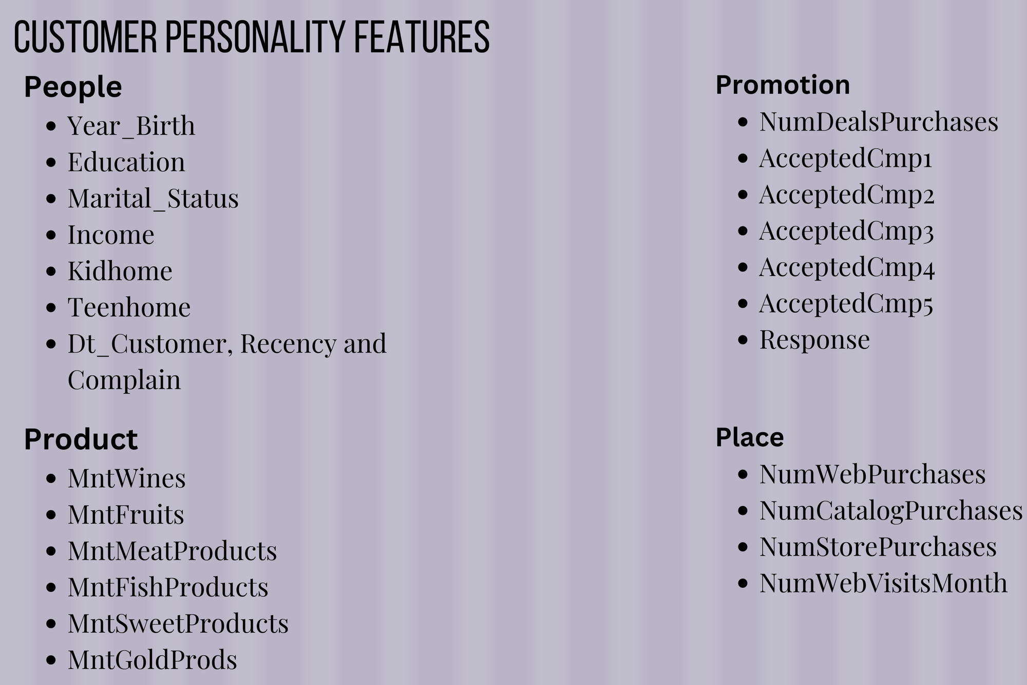
Customer Personality Analysis Features
| People | Promotion | Product | Place |
| Year Birth | NumberDealPurchase | MntWines | NumWebPurchases |
| Title | AcceptedCmp1 | MntFruits | NumCatalogPurchases |
| Education | AcceptedCmp2 | MntMeatProducts | NumStorePurchases |
| Marital_Status | AcceptedCmp3 | MntFishProducts | NumWebVisitsMonth |
| Income | AcceptedCmp4 | MntSweetProducts | |
| Kidhome | AcceptedCmp5 | MntGoldProds | |
| Teenhome | Response | ||
| Dt_customer, Recency, | |||
| and Complain |
To get the most out of this tutorial, you can download the entire Jupyter notebook beforehand so you can follow along easily. You can go here to fork the repo.
Exploratory Data Analysis (EDA)
As you might know, EDA is the key to performing well as a data analyst or data scientist. It gives you first-hand information about the whole dataset, and it helps you understand all the relationships between the features in your dataset.
We will perform the three phases of EDA in this tutorial which are:
Univariate Analysis.
Bivariate Analysis.
Multivariate Analysis
Firstly we need to import all the necessary libraries we will use in this project. We also need to load the dataset into a dataframe so we can see all the features that are present in it.
import pandas as pd
import seaborn as sns
import matplotlib.pyplot as plt
import plotly.express as px
import numpy as np
from scipy.stats import iqr
from sklearn.preprocessing import StandardScaler
from sklearn.cluster import KMeans


df = pd.read_csv("data/marketing_campaign.csv", sep="\t")
df.head()
To begin, there are many features in the dataset – but because we want to focus on customer demographics and behavior, we will only perform EDA on features related to those categories.
Keep in mind that the EDA conducted in this article is simply a subset of the one in the Jupyter Notebook. I did it this way to keep the article from becoming too buggy. To find the entire EDA in the notebook, fork the repo by clicking this link.
Age, income, marital status, education, total children, and amount spent on products are the attributes that belong to this category.
First, since the segmentation is based on the total amount customers have spent, we'll add the amount spent on the product:
df["TotalAmountSpent"] = df["MntFishProducts"] + df["MntFruits"] + df["MntGoldProds"] + df["MntSweetProducts"] + df["MntMeatProducts"] + df["MntWines"]
After that's done we can now begin our EDA. An effective EDA always has three stages, as I mentioned above. Again, they are as follows:
Univariate Analysis
Bivariate Analysis.
Multivariate Analysis.
Univariate analysis
Univariate analysis entails evaluating a single feature in order to get insights about it. So, the initial step in performing EDA is to undertake univariate analysis, which includes evaluating descriptive or summary statistics about the feature.
For example you might check a feature distribution, proportion of a feature, and so on.
In our case, we will check the distribution of customer's ages in the dataset. We can do that by typing the following:
sns.histplot(data=df, x="Age", bins = list(range(10, 150, 10)))
plt.title("Distribution of Customer's Age")

We can see from the above summary that most of the customers belong in the age range of 40-60.
Bivariate Analysis
After you've performed univariate analysis on all your feature of interest, the next step is to perform bivariate analysis. This involves comparing two attributes at the same time.
Bivariate analysis entails determining the correlation between two features, for example.
In our case, some of the bivariate analysis we'll perform in the project include observing the average total spent across different client age groups, determining a correlation between customer income and total amount spent, and so on, as shown below.
For example, in our case we want to check the relationship between a Customer's Income and TotalAmountSpent. We can do that by typing the following:
fig = px.scatter(data_frame=df_cut, x="Income",
                 y="TotalAmountSpent",
                 title="Relationship Between Customer's Income and Total Amount Spent",
                height=500,
                color_discrete_sequence = px.colors.qualitative.G10[1:])
fig.show()
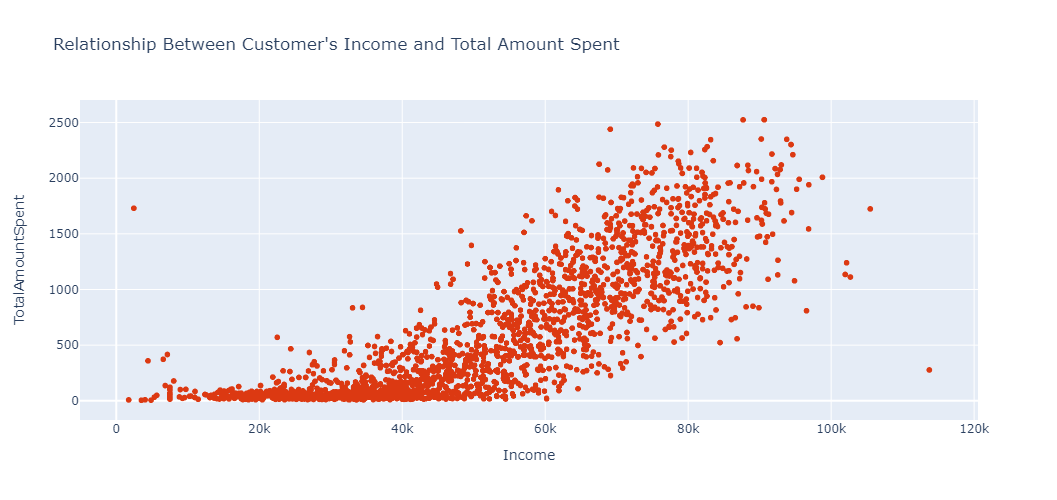
Analysis of relationship between customer's income and total amount spent.
We can see from the above analysis that as the Income increases so does the TotalAmountSpent. So from the analysis we can postulate that Income is one of key factor that determines how much a customer might spend.
Multivariate Analysis
After you've completed univariate (analysis of single feature) and bivariate (analysis of two features) analysis, the last phase of EDA is to perform Multivariate Analysis.
Multivariate Analysis consists of understanding the relationship between two or more variables.
In our project, one of the multivariate analysis we'll do is to understand the relationship between Income, TotalAmountSpent, and Customer's Education.
fig = px.scatter(
    data_frame=df_cut,
    x = "Income",
    y= "TotalAmountSpent",
    title = "Relationship between Income VS Total Amount Spent Based on Education",
    color = "Education",
    height=500
)
fig.show()
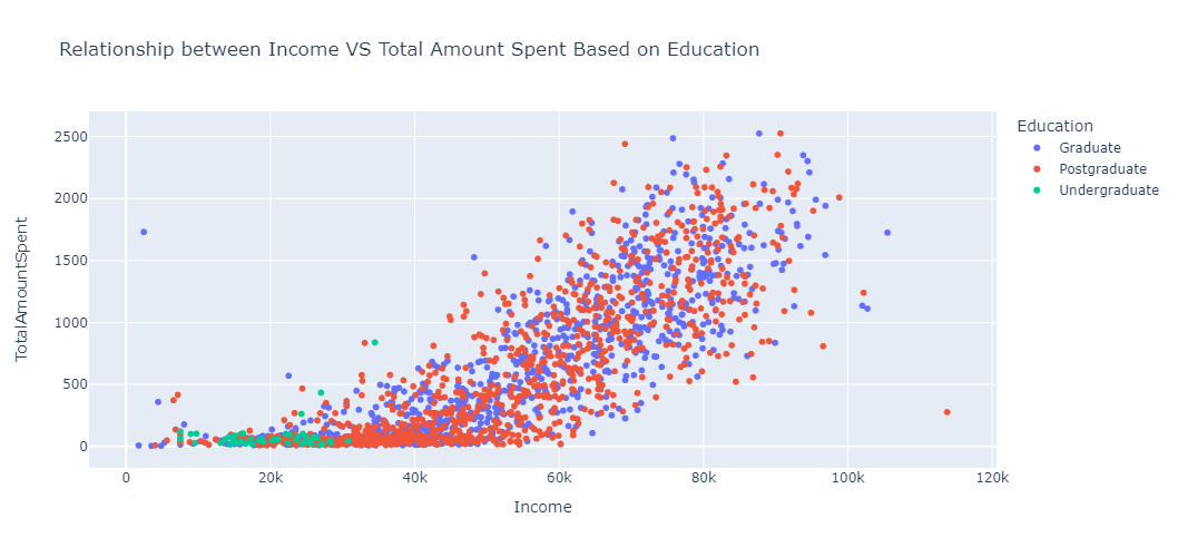
Analysis of relationship between income, total amount spent, and education.
We can see from the analysis that customers with an Undergraduate education level generally spend less than other customers with higher levels of education. This is because undergraduate customers typically earn less than other customers, which affects their spending habits.
How to Build the Segmentation Model
After we've finished our analysis, the next step is to create the model that will segment the customers. KMeans is the model we'll use. It is a popular segmentation model that is also quite effective.
The KMeans model is an unsupervised machine learning model that works by simply splitting N observations into K numbers of clusters. The observations are grouped into these clusters based on how close they are to the mean of that cluster, which is commonly referred to as centroids.
When you fit the features into the model and specify the number of clusters or segments you want, KMeans will output the cluster label to which each observation in the feature belongs.
Let's talk about the features you might want to fit into a KMeans model. There are no limits to the number of features you can use to build a Customer segmentation model – but in my opinion, fewer's better. This is because you will be able to grasp and interpret the outcomes of each segment more easily and clearly with fewer features.
In our scenario, we will first construct the KMeans model with two features and then build the final model with three features. But, before we get started, let's go over the KMeans assumptions, which are as follows:
The features must be numerical.
The features you're fitting into
KMeansmust be normally distributed. This is becauseKMeans(since it calculates average distance) is affected by outliers (values that deviate a lot from the others). As a result, any skewed feature must be changed in order to be normally distributed. Fortunately, we can use Numpy's logarithm transformation packagenp.log()The features must also be of the same scale. For this, we'll use the Scikit-learn
StandardScaler()module.
We'll design our KMeans model now that we've grasped the main concept. So, for our first model, we'll use the Income and TotalAmountSpent features.
To begin, because the Income feature has missing values, we will fill it with the median number.
df["Income"].fillna(df["Income"].median(), inplace=True)
After that, we'll assign the features we want to work with, Income and TotalAmountSpent, to a variable called data.
data = df[["Income", "TotalAmountSpent"]]
Once that's done we will transform features and save the result into a variable called data_log.
df_log = np.log(data)
Then we will scale the result using Scikit-learn StandardScaler():
std_scaler = StandardScaler()
df_scaled = std_scaler.fit_transform(df_log)
Once that's done we can then build the model. So the KMeans model requires two parameters. The first is random_state and the second one is n_clusterswhere:
n_clustersrepresents the number of clusters or segments to be derived fromKMeans.random_state: is required for reproducible results.
So, in a business setting, you might know the number of clusters you want to segment customers into ahead of time. But if not, you will need to experiment with different numbers of clusters to find the optimal one.
Since we're not in a business setting, we will experiment with different numbers of clusters.
The elbow method is the strategy we'll use to select the best cluster. It works simply by plotting the error from each cluster and looking for a spot that forms an elbow on the plot. As a result, the ideal cluster is the one that produces that elbow.
Here's the code that will help us achieve that:
errors = []
for k in range(1, 11):
    model = KMeans(n_clusters=k, random_state=42)
    model.fit(df_scaled)
    error.append(model.inertia_)


plt.title('The Elbow Method')
plt.xlabel('k'); plt.ylabel('Error of Cluster')
sns.pointplot(x=list(range(1, 11), y=errors)
plt.show()
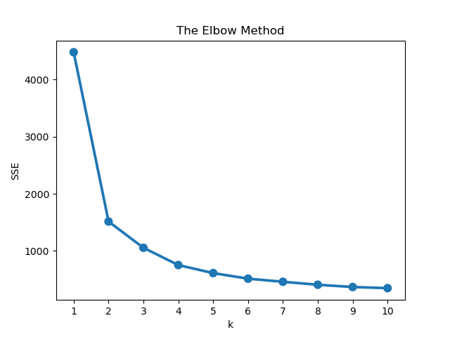
Let's summarize what the above code does. We specified the number of clusters to experiment with, which is in the range(1, 11). Then we fit the features on those clusters and added the error to the list we created before above.
Following that, we plot the error for each cluster. The diagram shows that the cluster that creates the elbow is three. So three clusters is the best value for our model. As a result, we will build the KMeans model utilizing three clusters.
model = KMeans(n_clusters = 3, random_state=42)
model.fit(df_scaled)
Now we've built our model. The next thing will be to assign the cluster label for each observation. So we will assign the label to the original feature we didn't processed. That is, where we assigned Income and TotalAmountSpent to the variable data
data = data.assign(ClusterLabel = model.labels_)
How to Interpret the Cluster Result
Now that we've built the model, the next thing will be to interpret the result from each cluster.
There are numerous way you can summarize the results of your cluster depending on what you want to achieve. The most common summary is using central tendency which includes mean, median, and mode.
For our case we will make use of median. We're using median because the original features have outliers and the mean is very sensitive to outliers.
So we will aggregate the cluster labels and find the median for Income and TotalAmountSpent. We can make use of Pandas groupby method for that.
data.groupby("ClusterLabel")[["Income", "TotalAmountSpent"]].median()

We can see that there is a trend within the clusters:
Cluster 0 translates to customers who earn less and spend less.
Cluster 1 represent customers that earn more and spend more.
Cluster 2 represents customers that earn moderate and spend moderate.
We can also visualize the relationship by entering the following code:
fig = px.scatter(
    data_frame=data,
    x = "Income",
    y= "TotalAmountSpent",
    title = "Relationship between Income VS Total Amount Spent",
    color = "ClusterLabel",
    height=500
)
fig.show()
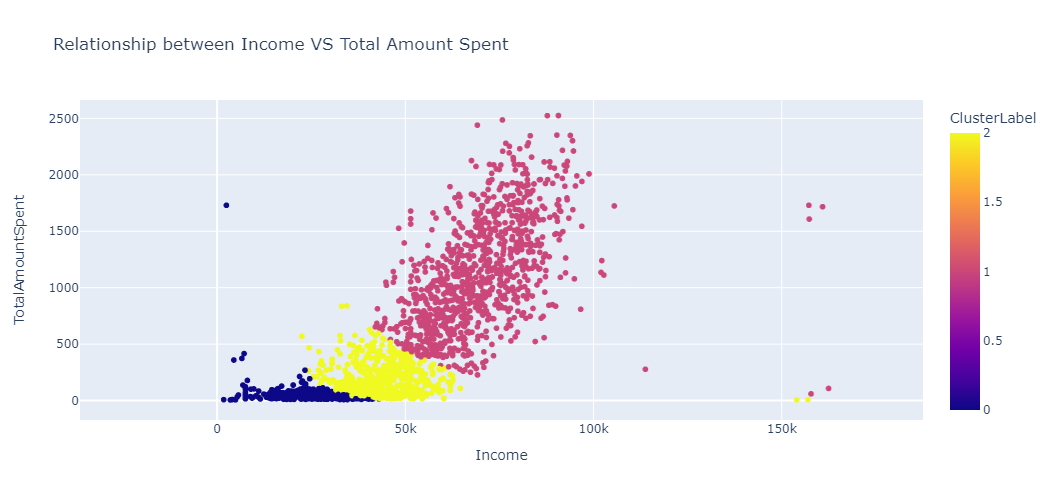
Analysis of relationship between income and total amount spent
Now in the same way we built the formal model, we will build the KMeans model using 3 features (the elbow method also depicts that 3 clusters is the optimal one).
data = df[["Age", "Income", "TotalAmountSpent"]]
df_log = np.log(data)
std_scaler = StandardScaler()
df_scaled = std_scaler.fit_transform(df_log)
model = KMeans(n_clusters=3, random_state=42)
model.fit(df_scaled)

data = data.assign(ClusterLabel= model.labels_)

result = df_result.groupby("ClusterLabel").agg({"Age":"mean", "Income":"median", "TotalAmountSpent":"median"}).round()

We can see from the above summary that:
Cluster 0 depicts young customers that earn a lot and also spend a lot.
Cluster 1 translates to older customers that earn a lot and also spend a lot.
Cluster 2 depicts young customers that earn less and also spend less.
We can also visualize our result by typing the following code:
fig = px.scatter_3d(data_frame=data, x="Income",
                    y="TotalAmountSpent", z="Age", color="ClusterLabel", height=550,
                   title = "Visualizing Cluster Result Using 3 Features")
fig.show()
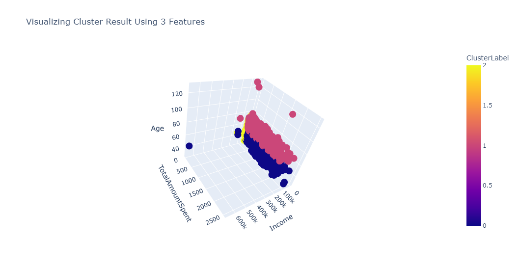
Cluster results using three features
Conclusion
In this tutorial, you learnt how to build a customer segmentation model. There are a lot of features we didn't touch on in this article. But I suggest that you experiment with it and create customer segmentation models using different features.
I hope you learn more from doing that. Thank you for reading the article. Happy Coding!
The link to the full code can be found below. And here's an article on K-Means Clustering if you want to learn more.