
By Tirthajyoti Sarkar
In this article, we discuss 8 ways to perform simple linear regression using Python code/packages. We gloss over their pros and cons, and show their relative computational complexity measure.
For many data scientists, linear regression is the starting point of many statistical modeling and predictive analysis projects. The importance of fitting (accurately and quickly) a linear model to a large data set cannot be overstated. As pointed out in this article, ‘LINEAR’ term in the linear regression model refers to the coefficients, and not to the degree of the features.
Features (or independent variables) can be of any degree or even transcendental functions like exponential, logarithmic, sinusoidal. Thus, a large body of natural phenomena can be modeled (approximately) using these transformations and linear model even if the functional relationship between the output and features are highly nonlinear.
On the other hand, Python is fast emerging as the de-facto programming language of choice for data scientists. Therefore, it is critical for a data scientist to be aware of all the various methods he/she can quickly fit a linear model to a fairly large data set and asses the relative importance of each feature in the outcome of the process.
However, is there only one way to perform linear regression analysis in Python? In case of multiple available options, how to choose the most effective method?
Because of the wide popularity of the machine learning library scikit-learn, a common approach is often to call the Linear Model class from that library and fit the data. While this can offer additional advantages of applying other pipeline features of machine learning (e.g. data normalization, model coefficient regularization, feeding the linear model to another downstream model), this is often not the fastest or cleanest method when a data analyst needs just a quick and easy way to determine the regression coefficients (and some basic associated statistics).
There are faster and cleaner methods. But all of them may not offer same amount of information or modeling flexibility.
Please read on.
The entire boiler plate code for various linear regression methods is available here on my GitHub repository. Most of them are based on the SciPy package.
SciPy is a collection of mathematical algorithms and convenience functions built on the Numpy extension of Python. It adds significant power to the interactive Python session by providing the user with high-level commands and classes for manipulating and visualizing data.
Let me discuss each method briefly,
Method: Scipy.polyfit( ) or numpy.polyfit( )
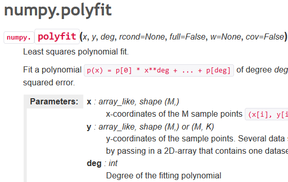
This is a pretty general least squares polynomial fit function which accepts the data set and a polynomial function of any degree (specified by the user), and returns an array of coefficients that minimizes the squared error. Detailed description of the function is given here. For simple linear regression, one can choose degree 1. If you want to fit a model of higher degree, you can construct polynomial features out of the linear feature data and fit to the model too.
Method: Stats.linregress( )
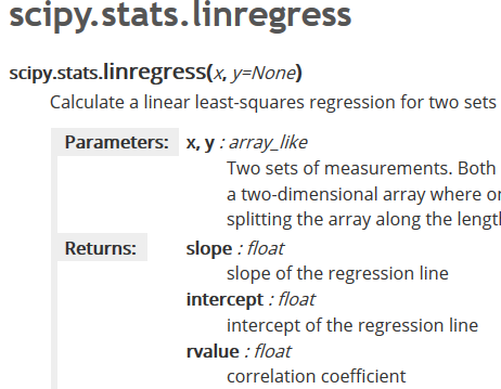
This is a highly specialized linear regression function available within the stats module of Scipy. It is fairly restricted in its flexibility as it is optimized to calculate a linear least-squares regression for two sets of measurements only. Thus, you cannot fit a generalized linear model or multi-variate regression using this. But, because of its specialized nature, it is one of the fastest method when it comes to simple linear regression. Apart from the fitted coefficient and intercept term, it also returns basic statistics such as R² coefficient and standard error.
Method: Optimize.curve_fit( )
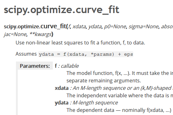
This is along the same line as Polyfit method, but more general in nature. This powerful function from scipy.optimize module can fit any user-defined function to a data set by doing least-square minimization.
For simple linear regression, one can just write a linear mx+c function and call this estimator. Goes without saying that it works for multi-variate regression too. It returns an array of function parameters for which the least-square measure is minimized and the associated covariance matrix.
Method: numpy.linalg.lstsq
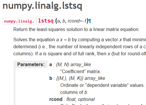
This is the fundamental method of calculating least-square solution to a linear system of equation by matrix factorization. It comes from the handy linear algebra module of numpy package. Under the hood, it solves the equation a x = b by computing a vector x that minimizes the Euclidean 2-norm || b — a x ||².
The equation may be under-, well-, or over- determined (i.e., the number of linearly independent rows of a can be less than, equal to, or greater than its number of linearly independent columns). If a is square and of full rank, then x (but for round-off error) is the “exact” solution of the equation.
You can do either simple or multi-variate regression with this and get back the calculated coefficients and residuals. One little trick is that before calling this function you have to append a column of 1’s to the x data to calculate the intercept term. Turns out it is one of the faster methods to try for linear regression problems.
Method: Statsmodels.OLS ( )
Statsmodels is a great little Python package that provides classes and functions for the estimation of many different statistical models, as well as for conducting statistical tests, and statistical data exploration. An extensive list of result statistics are available for each estimator. The results are tested against existing statistical packages to ensure correctness.
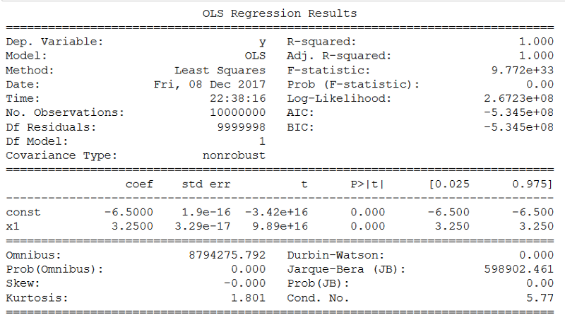
For linear regression, one can use the OLS or Ordinary-Least-Square function from this package and obtain the full blown statistical information about the estimation process.
One little trick to remember is that you have to add a constant manually to the x data for calculating the intercept, otherwise by default it will report the coefficient only. Below is the snapshot of the full results summary of the OLS model. It is as rich as any functional statistical language like R or Julia.
Method: Analytic solution using matrix inverse method
For well-conditioned linear regression problems (at least where # of data points > # of features), a simple closed-form matrix solution exists for calculating the coefficients which guarantees least-square minimization. It is given by,
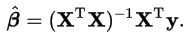
Detailed derivation and discussion about this solution is discussed here.
One has two choices here:
(a) using simple multiplicative matrix inverse.
(b) first computing the Moore-Penrose generalized pseudoinverse matrix of x-data followed by taking a dot product with the y-data. Because this 2nd process involves singular-value decomposition (SVD), it is slower but it can work for not well-conditioned data set well.
Method: sklearn.linear_model.LinearRegression( )
This is the quintessential method used by majority of machine learning engineers and data scientists. Of course, for real world problem, it is probably never much used and is replaced by cross-validated and regularized algorithms such as Lasso regression or Ridge regression. But the essential core of those advanced functions lies in this model.
Measuring speed and time complexity of these methods
As a data scientist, one should always look for accurate yet fast methods/function to do the data modeling work. If the method is inherently slow, then it will create execution bottleneck for large data sets.
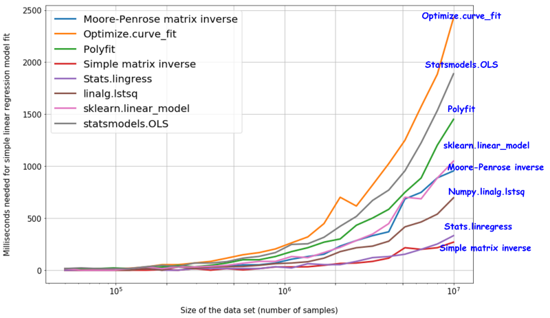
A good way to determine scalability is to run the models for increasing data set size, extract the execution times for all the runs and plot the trend.
Here is the boiler plate code for this. And here is the result. Due to their simplicity, stats.linregress and simple matrix inverse methods are fastest, even up to 10 million data points.
Summary
As a data scientist, one must always explore multiple options for solving the same analysis or modeling task and choose the best for his/her particular problem.
In this article, we discussed 8 ways to perform simple linear regression. Most of them are scalable to more generalized multi-variate and polynomial regression modeling too. We did not list the R² fit for these methods as all of them are very close to 1.
For a single-variable regression, with millions of artificially generated data points, the regression coefficient is estimated very well.
The goal of this article is primarily to discuss the relative speed/computational complexity of these methods. We showed the computational complexity measure of each of them by testing on a synthesized data set of increasing size (up to 10 million samples). Surprisingly, the simple matrix inverse analytic solution works pretty fast compared to scikit-learn’s widely used Linear Model.
If you have any questions or ideas to share, please contact the author at tirthajyoti[AT]gmail.com. Also you can check author’s GitHub repositories for other fun code snippets in Python, R, or MATLAB and machine learning resources. If you are, like me, passionate about machine learning/data science/semiconductors, please feel free to add me on LinkedIn or follow me on Twitter.