
Welcome to the Databricks Delta Lake with SQL Handbook! Databricks is a unified analytics platform that brings together data engineering, data science, and business analytics into a collaborative workspace.
Delta Lake, a powerful storage layer built on top of Databricks, provides enhanced reliability, performance, and data quality for big data workloads.
This is a hands-on training guide where you will get a chance to dive into the world of Databricks and learn how to effectively use Delta Lake for managing and analyzing data. It'll provide you with the essential SQL skills to efficiently interact with Delta tables and perform advanced data analytics.
Prerequisites
This handbook is designed for beginner-level SQL users who have some experience with cloud platforms and clusters. Although no prior experience with Databricks is required, it is recommended that you have a basic understanding of the following concepts:
Databases: Familiarity with the basic structure and functionality of databases will be helpful.
SQL Queries: Knowledge of SQL syntax and the ability to write basic queries is essential.
Jupyter Notebooks: Understanding how Jupyter notebooks work and being comfortable with running code cells is recommended.
While this handbook assumes a certain level of familiarity with databases, SQL, and Jupyter notebooks, it will guide you step-by-step through each process, ensuring that you understand and follow along with the material.
As such, no installation is necessary, as all the work will be done on Databricks Delta Notebooks running in the cluster. Everything has already been provisioned, eliminating the need for any setup or configuration.
By the end of this handbook, you would have gained a solid foundation in using SQL with Databricks, enabling you to leverage its powerful capabilities for data analysis and manipulation.
Let's get started!
Table of Contents
Here are the sections of this tutorial:
What is Databricks?
Key features and benefits
Getting started with Databricks Workspace
Notebook basics and interactive analytics
Understanding Delta Lake
Advantages of using Delta
Use cases of Delta in real-world scenarios
Supported languages and platforms for Delta
Creating tables from various data sources
SQL Data Definition Language (DDL) commands
SQL Data Manipulation Language (DML) commands
Creating tables from a Databricks dataset
Saving the loaded CSV file to Delta using Python
Delta SQL commands for data management
Performing UPSERT (UPDATE and INSERT) operations
Handling data visualization in Delta
Advanced aggregate queries in Delta
Counting diamonds by clarity using SQL
Adding table constraints for data integrity
Creating a DataFrame from a Databricks dataset
Data manipulation and displaying results using DataFrames
Understanding version control and time travel in Delta
Restoring data to a specific version
Utilizing autogenerated fields for metadata tracking
Deep and shallow copying of Delta tables
Efficiently cloning Delta tables for data exploration and analysis
Introduction to Databricks
Databricks is a unified analytics platform that combines data engineering, data science, and machine learning into a single collaborative environment. Leveraging Apache Spark, it processes and analyzes vast amounts of data efficiently.
Databricks offers benefits like seamless scalability, real-time collaboration, and simplified workflows, making it a favored choice for data-driven enterprises.
Its versatility suits various use cases: from ETL processes and data preparation to advanced analytics and AI model development. Databricks aids in uncovering insights from structured and unstructured data, empowering businesses to make informed decisions swiftly.
You can see its application in finance for fraud detection, healthcare for predictive analytics, e-commerce for recommendation engines, and so on. Basically, Databricks accelerates data-driven innovation, transforming raw information into actionable intelligence.
To follow along this tutorial, you should first create a Community Edition account so you can create your clusters.
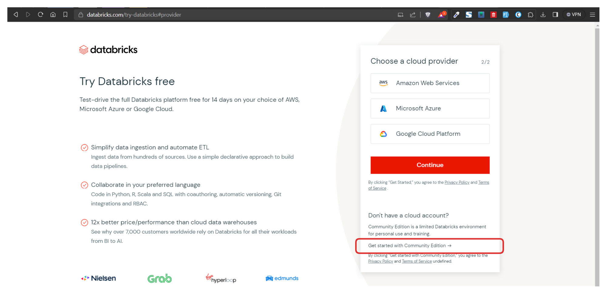
Create a Databricks Community Edition Account
Once you've created your account, head over to the Community Edition login page. Once you have signed in, you'll be greeted with a screen very similar to the one shown below.
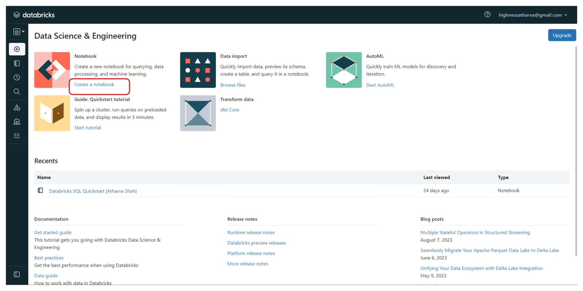
Databricks User Dashboard with options to create workspaces, notebooks, and import data
From the sidebar on the left, you can create your workspaces, and upload datasets and files that you wish to process.
To follow along, click on the link highlighted in the image above (the one that says "create a notebook"). It will launch a new notebook on Databricks platform where we'll be writing all the code.
You can also access all your notebooks from the left sidebar or from the "Recents" tab on the home screen once you login.
You can find all the code, instructions, and steps used in this handbook with explanations in one of the public notebooks I have created here.
On creating a new notebook, you should create a cluster to run your commands and process the data. Clusters in the Databricks Delta platform are groups of computing resources that drive efficient data processing. They execute tasks in parallel, speeding up tasks like ETL and analysis.
Clusters offer tailored resource allocation, ensuring optimal performance and scalability. Supporting multiple users and tasks concurrently, clusters encourage collaboration. Leveraging Apache Spark, they enable advanced analytics and machine learning.
Integral to Databricks Delta's ACID transactions, clusters ensure data integrity. Overall, clusters empower seamless, high-performance data handling, essential for tasks ranging from data preparation to sophisticated analytics and AI model training.

Provision a cluster by creating a new resource to run commands in the notebook

Proceed with the standard configuration
Now that we have the notebook and clusters set up, we can start with the code. But before we do that, here are a few key terms to know. Awareness of these is more about the platform and less about SQL syntax which will be covered below.
Data Ingestion
Data ingestion in Delta involves loading data from third-party sources, such as Fivetran. The most efficient storage medium for data in Delta is Parquet, which is a columnar storage format. To load data into Delta, we can use Spark or PySpark Python and specify the storage location. The loaded data can be accessed and queried using SQL syntax with the COPY INTO command.
Dashboards
Visualizations created in SQL notebooks within Delta can be added to custom dashboards for BI/Analytics. These dashboards are lightweight and provide real-time updates based on data refreshment. This enables users to create insightful and interactive dashboards for data analysis and reporting. You need not create your dashboards from scratch. Popular Dashboard templates are available.
Policies
Delta provides data governance through the Unity Catalog, ensuring that users only have access to databases and tables they are permitted to view or edit. This granular control over data access enhances security and data privacy within the system.
History
Moderators or superusers can access the history of each query run against all databases, along with timestamps and query execution times. This feature helps in understanding query patterns and optimizing database performance based on usage insights.
Optimization
To improve query performance, Delta offers various optimization techniques, such as database indexing, clustering, Bloom filter indexing, and leveraging MPP paradigms like MapReduce. Knowledge of normalization and schema design also contributes to writing efficient SQL queries.
Alerts
Delta allows users to set alerts based on comparison operators applied to query results. For example, when a sales count query returns a value below a threshold, an alert can be triggered via Slack, ticketing tools, or emails. Customizable alerts ensure timely notifications for critical data events.
Persona-Based Design
The Databricks Platform is designed to cater to different personas, including Data Science/Analytics and BI/MLOps specialists. Users get segregated interfaces tailored to their roles. However, the Unity Catalog can aggregate all these views, providing a cohesive experience.
SQL Workspace
The SQL Workspace in Delta provides an interface similar to MySQL Workbench or PgAdmin. Users can perform SQL queries on datasets without the need to load the data repeatedly, as done in notebooks. This efficient querying enhances the SQL-based data analysis experience.
Integration with other BI Tools
Databricks integrates well with Tableau and PowerBI. You can import your data points and visualizations seamlessly and get consistent and synced results in the BI tools of your choice. With the click of a button, live queries are generated against the Databricks datasets.
Introduction to Delta
Delta Lake is an open storage format used to save your data in your Lakehouse. Delta provides an abstraction layer on top of files. It's the storage foundation of your Lakehouse.
Why Delta Lake?
![]()
Running an ingestion pipeline on Cloud Storage can be very challenging. Data teams typically face the following challenges:
Hard to append data (Adding newly arrived data leads to incorrect reads).
Modification of existing data is difficult (GDPR/CCPA requires making fine-grained changes to the existing data lake).
Jobs failing mid-way (Half of the data appears in the data lake, the rest may be missing).
Data quality issues (It’s a constant headache to ensure that all the data is correct and high quality).
Real-time operations (Mixing streaming and batch leads to inconsistency).
Costly to keep historical versions of the data (Regulated environments require reproducibility, auditing, and governance).
Difficult to handle large metadata (For large data lakes, the metadata itself becomes difficult to manage).
“Too many files” problems (Data lakes are not great at handling millions of small files).
Hard to get great performance (Partitioning the data for performance is error-prone and difficult to change).
These challenges have a real impact on team efficiency and productivity, spending unnecessary time fixing low-level, technical issues instead of focusing on high-level, business implementation.
Because Delta Lake solves all the low-level technical challenges of saving petabytes of data in your lakehouse, it lets you focus on implementing a simple data pipeline while providing blazing-fast query answers for your BI and analytics reports.
In addition, Delta Lake is a fully open source project under the Linux Foundation and is adopted by most of the data players. You know you own your data and won't have vendor lock-in.
Features and Capabilities
You can think about Delta as a file format that your engine can leverage to bring the following capabilities out of the box:
ACID transactions
Support for DELETE/UPDATE/MERGE
Unify batch & streaming
Time Travel
Clone zero copy
Generated partitions
CDF - Change Data Flow (DBR runtime)
Blazing-fast queries
This hands-on quickstart guide is going to focus on:
Loading Databases and Tabular Data from a variety of sources
Writing DDL, DML, and DTL queries on these datasets
Visualizing Datasets to get conclusive results
Time travel and Restoring database
Performance Optimization
How to Create and Manage Tables
Okay, time to code! If you still have the notebook that we created earlier along with the clusters open, you can start by following along with the code below. Don't worry, explanations for every step will follow.
Select the dropdown next to the notebook title and ensure SQL is selected since this handbook is all about Delta Lakes with SQL.

Select Notebook language to be SQL
How to Create Tables from a Databricks Dataset
Databricks notebooks are very much like Jupyter Notebooks. You have to insert your code into cells and run them one by one or together. All the output is shown cell by cell, progressively.
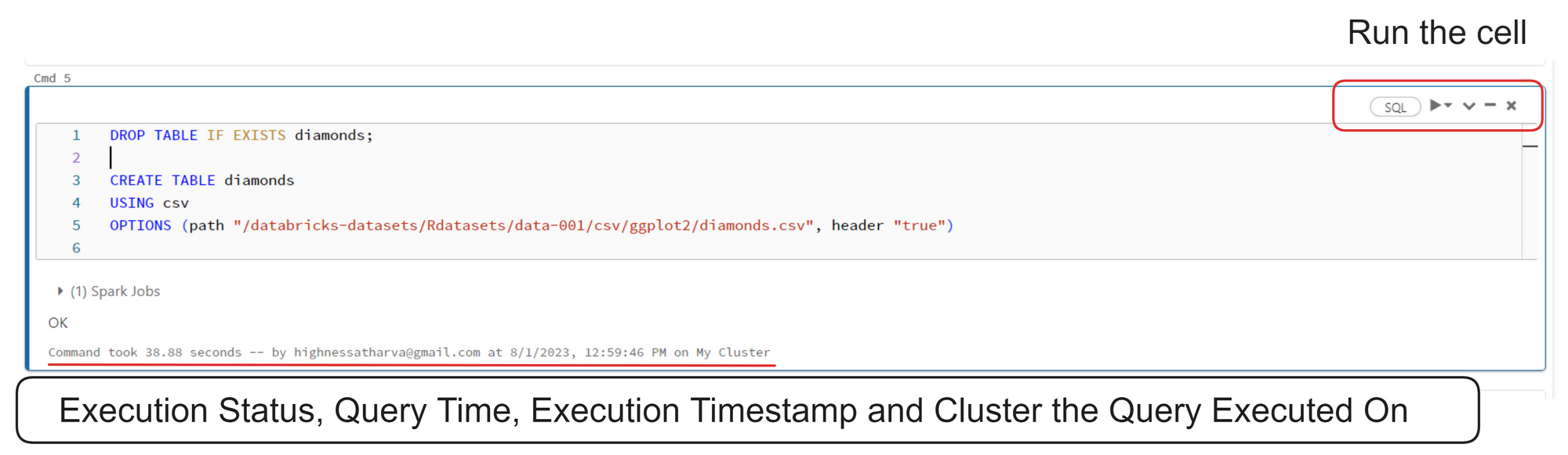
Databricks notebook interface
Here's the code from the image above:
DROP TABLE IF EXISTS diamonds;
CREATE TABLE diamonds
USING csv
OPTIONS (path "/databricks-datasets/Rdatasets/data-001/csv/ggplot2/diamonds.csv", header "true")
In the code above, the two SQL statements (CREATE TABLE) are used to create a table named diamonds in a database. The table is based on data from a CSV file located at the specified path.
If a table with the same name already exists, the DROP TABLE IF EXISTS diamonds statement ensures it is deleted before creating a new one. The table will have the same schema as the CSV file, with the first row assumed to be the header containing column names ("header 'true'").
Here's a command that returns all the records from the diamonds table:
SELECT * from diamonds

The above query returns all the records from the diamonds table
Here's another command:
describe diamonds;

Table metadata returned by the describe command
In SQL, the DESCRIBE statement is used to retrieve metadata information about a table's structure. The specific syntax for the DESCRIBE statement can vary depending on the database system being used.
However, its primary purpose is to provide details about the columns in a table, such as their names, data types, constraints, and other properties.
Saving the loaded CSV file to Delta using Python
The best part about using the Databricks platform is that it allows you to write Python, SQL, Scala, and R interchangeably in the same notebook.
You can switch up the languages at any given point by using the "Delta Magic Commands". You can find a full list of magic commands at the end of this handbook.
%python

diamonds = spark.read.csv("/databricks-datasets/Rdatasets/data-001/csv/ggplot2/diamonds.csv", header="true", inferSchema="true")

diamonds.write.format("delta").mode("overwrite").save("/delta/diamonds")
Data is read from a CSV file located at /databricks-datasets/Rdatasets/data-001/csv/ggplot2/diamonds.csv into a Spark DataFrame named diamonds. The first row of the CSV file is treated as the header, and Spark infers the schema for the DataFrame based on the data.
The DataFrame diamonds is written in a Delta Lake table format. If the table already exists at the specified location (/delta/diamonds), it will be overwritten. If it does not exist, a new table will be created.
DROP TABLE IF EXISTS diamonds;

CREATE TABLE diamonds USING DELTA LOCATION '/delta/diamonds/'
The SQL statements above drops any existing table named diamonds and creates a new Delta Lake table named diamonds using the data stored in the Delta Lake format at the /delta/diamonds/ location.
You can run a SELECT statement to ensure that the table appears as expected:
SELECT * from diamonds

The same diamonds table result set once restored from Delta Lake
Delta SQL Command Support
In the world of databases, there are two fundamental types of commands: Data Manipulation Language (DML) and Data Definition Language (DDL). These commands play a crucial role in managing and organizing data within a database. In this article, we will explore what DML and DDL commands are, their key differences, and provide examples of how they are used.
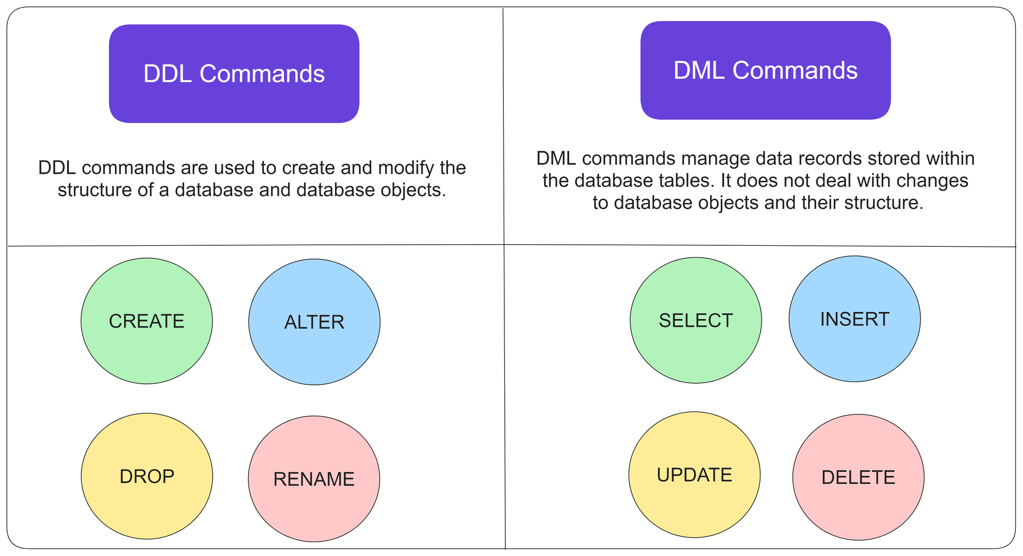
Databricks Notebooks support all the SQL commands including DDL and DML commands highlighted here
Data Manipulation Language (DML)
It is used to manipulate or modify data stored in a database. These commands allow users to insert, retrieve, update, and delete data from database tables. Let's take a closer look at some commonly used DML commands:
SELECT: The SELECT command is used to retrieve data from one or more tables in a database. It allows you to specify the columns and rows you want to extract by using conditions and filters. For example, SELECT * FROM Customers retrieves all the records from the Customers table.
INSERT: The INSERT command adds new data into a table. It allows you to specify the value for each column or select values from another table. For example, INSERT INTO Customers (Name, Email) VALUES ('John Doe', 'john@example.com') adds a new customer record to the Customers table.
UPDATE: The UPDATE command is used to modify existing data in a table. It allows you to change the values of specific columns based on certain conditions. For example, UPDATE Customers SET Email = 'new@example.com' WHERE ID = 1 updates the email address of the customer with ID of 1.
DELETE: The DELETE command is used to remove data from a table. It allows you to delete specific rows based on certain conditions. For example, DELETE FROM Customers WHERE ID = 1 deletes the customer record with ID of 1 from the Customers table.
Data Definition Language (DDL) Commands
DDL commands are used to define the structure and organization of a database. These commands allow users to create, modify, and delete database objects such as tables, indexes, and constraints.
Let's explore some commonly used DDL commands:
CREATE: Creates a new database object, such as a table or an index. It allows you to define the columns, data types, and constraints for the object. For example, CREATE TABLE Customers (ID INT, Name VARCHAR(50), Email VARCHAR(100)) creates a new table named Customers with three columns.
ALTER: Modifies the structure of an existing database object. It allows you to add, modify, or delete columns, constraints, or indexes. For example, ALTER TABLE Customers ADD COLUMN Phone VARCHAR(20) adds a new column named Phone to the Customers table.
DROP: Deletes an existing database object. It permanently removes the object and its associated data from the database. For example, DROP TABLE Customers deletes the Customers table from the database.
TRUNCATE: The TRUNCATE command is used to remove all the data from a table, while keeping the table structure intact. It is faster than the DELETE command when you want to remove all records from a table. For example, TRUNCATE TABLE Customers removes all records from the Customers table.
Delta Lake supports standard DML including UPDATE, DELETE and MERGE INTO, providing developers with more control to manage their big datasets.
Here's an example that uses the INSERT, UPDATE, and SELECT commands:
INSERT INTO diamonds(_c0, carat, cut,    color,    clarity,    depth,    table,    price,    x,    y,    z) values (53941, 0.22,    'Premium', 'I',    'SI2',    '60.3',    '62.1',    '334',    '3.79',    '3.75',    '2.27');

UPDATE diamonds SET carat = 0.20 WHERE _c0 = 53941;

select * from diamonds where _c0=53941;
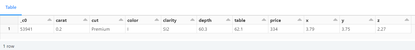
Fetching a unique record from the table
In the example above, an initial row is inserted into the diamonds table with specific values for each column.
Then the carat value for the row with _c0 equal to 53941 is updated to 0.20.
The final SELECT statement retrieves the row with _c0 equal to 53941, showing its current state after the INSERT and UPDATE operations. This shows that the record insertion was successful.
DELETE FROM diamonds where _c0=53941;

select * from diamonds where _c0=53941;
The above DELETE command paired with the WHERE clause removes the row from the database and the subsequent SELECT query validates this by returning a null result set.
UPSERT Operation
The "upsert" operation updates if the record exists, and inserts the record doesn't exist.
CREATE TABLE  diamond__mini(_c0 int, carat double, cut string,    color string,    clarity string,    depth double, table double,    price int,    x double,    y double,    z double);

delete from diamond__mini;

INSERT INTO diamond__mini(_c0, carat, cut,    color,    clarity,    depth,    table,    price,    x,    y,    z) values (1, 0.22,    'Premium', 'I',    'SI2',    '60.3',    '62.1',    '334',    '3.79',    '3.75',    '2.27');
INSERT INTO diamond__mini(_c0, carat, cut,    color,    clarity,    depth,    table,    price,    x,    y,    z) values (2, 0.22,    'Premium', 'I',    'SI2',    '60.3',    '62.1',    '334',    '3.79',    '3.75',    '2.27');
INSERT INTO diamond__mini(_c0, carat, cut,    color,    clarity,    depth,    table,    price,    x,    y,    z) values (90000, 0.22,    'Premium', 'I',    'SI2',    '60.3',    '62.1',    '334',    '3.79',    '3.75',    '2.27');

select * from diamond__mini;
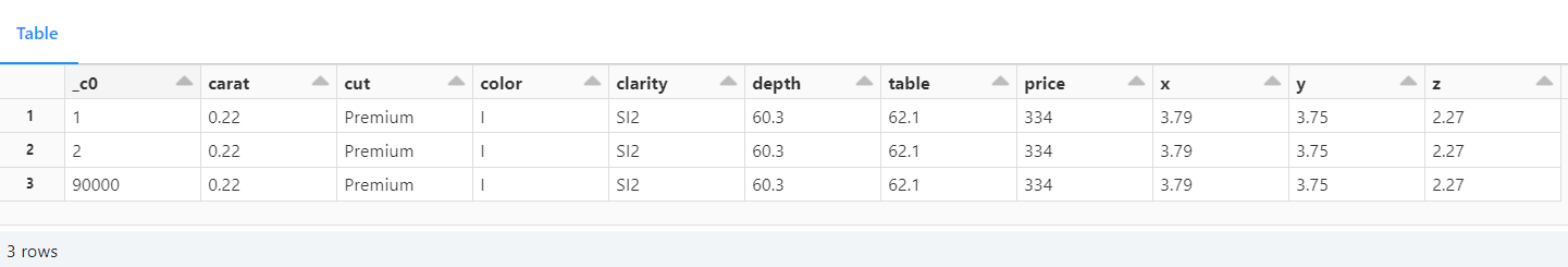
Creating a subset diamonds_mini to demonstrate the UPSERT operation
In this scenario, we have created a table named diamond__mini to test upsert (that is, insert or update) operations into the diamonds table.
diamond__mini is a subset of the diamonds table, containing only 3 records. Two of these rows (with _c0 values 1 and 2) already exist in the diamonds table, and one row (with _c0 value 90000) does not exist.
Therefore, the code will drop and create the diamond__mini table with a specific schema to match the diamonds table.
Then clear the diamond__mini table by deleting all existing records, ensuring that we have a clean slate for the upsert test.
It'll then perform three INSERT statements to the diamond__mini table, attempting to add three new records with different _c0 values, including one with _c0 = 90000.
Lastly, we'll select all records from the diamond__mini table to observe the changes and verify if the upsert worked correctly.
Since the _c0 values 1 and 2 already exist in the diamonds table, the corresponding rows in diamond__mini will be considered as updates for the existing rows.
On the other hand, the row with _c0 = 90000 is new and does not exist in the diamonds table, so it will be treated as an insert.
The describe command shows the metadata of the new table:
describe diamond__mini
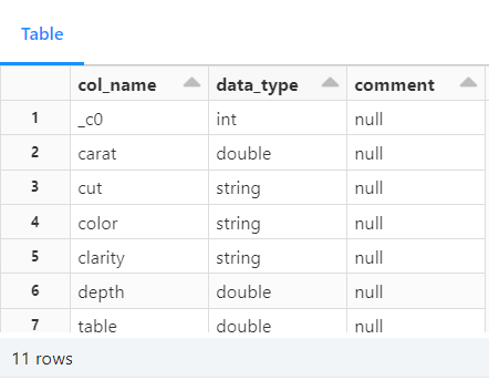
Fetching metadata of the newly created table
Here's another example that uses the upsert operation:

upsert operation on diamond and diamond_mini tables
-- perform UPSERT operation based on matching column and row criteria from diamond__mini to diamonds table. If a match is found, record will update otherwise it will be inserted.

MERGE INTO diamonds as d USING diamond__mini as m
  ON d._c0 = m._c0
  WHEN MATCHED THEN
    UPDATE SET *
  WHEN NOT MATCHED
    THEN INSERT * ;

select * from diamonds where _c0 in (1 ,2, 90000)

UPSERT operation successful. Values for records with _c0 = [1,2] were updated and 90,000 was inserted
In this example, a MERGE operation is performed between two tables: diamonds (target table) and diamond__mini (source table). The MERGE statement compares the records in both tables based on the common _c0 column.
Here's a concise explanation:
The
MERGEstatement matches records with the same_c0value in both tables (diamondsanddiamond__mini).When a match is found (based on
_c0), it performs anUPDATEon the target table (diamonds) using the values from the source table (diamond__mini). This is done for all columns usingUPDATE SET *.If no match is found for a record from the source table (
diamond__mini), it performs anINSERTinto the target table (diamonds) using the values from the source table for all columns (usingINSERT *).After the
MERGEoperation, aSELECTstatement retrieves the records from the target table (diamonds) with _c0 values 1, 2, and 90000 to observe the changes made during the merge.
The MERGE statement is used to synchronize data between the diamondsand diamond__mini tables based on their common _c0column, updating existing records and inserting new ones.
Advanced SQL Queries
Data Visualization in Delta
In Databricks Delta platform, you can leverage SQL queries to visualize data and gain valuable insights without the need for complex programming. Here are some ways to visualize data using SQL queries in Databricks Delta:
Basic SELECT Queries: Retrieves data from your Delta tables. By selecting specific columns or applying filters with WHERE clauses, you can quickly get an overview of the data's characteristics.
Aggregate Functions: SQL provides a variety of aggregate functions like
COUNT,SUM,AVG,MIN, andMAX. By using these functions, you can summarize and visualize data at a higher level. You perform operations such as counting the number of records, calculating the average values, or finding the maximum and minimum values.Grouping and Aggregating Data: The
GROUP BYclause in SQL allows you to group data based on specific columns, and then apply aggregate functions to each group. This enables generation of meaningful insights by analyzing data on a category-wise basis.Window Functions: SQL window functions, like
ROW_NUMBER,RANK, andDENSE_RANK, are valuable for partitioning data and calculating rankings or running totals. These functions enable analyzing data in a more granular way and help discover patterns.Joining Tables: Helps to combine data from multiple Delta tables using SQL
JOINoperations. Merging related data, performing cross-table analysis, and advanced visualizations is possible through joins.Subqueries and CTEs: SQL subqueries and Common Table Expressions (CTEs) allow you to break down complex problems into manageable parts. These techniques can simplify analysis and make SQL queries more organized and maintainable.
Window Aggregates: SQL window aggregates, such as
SUM,AVG, andROW_NUMBERwith theOVERclause, enable you to perform calculations on specific windows or ranges of data. This is useful for analyzing trends over time or within specific subsets of your data.CASE Statements: CASE statements in SQL help you create conditional expressions, allowing you to categorize or group data based on certain conditions. This can aid in creating custom labels or grouping data into different categories for visualization purposes.
The platform's powerful SQL capabilities empower data analysts and developers to extract meaningful insights from their Delta Lake data, all without the need for additional programming languages or tools.
-- aggregate query to get average price based on diamond colors
SELECT color, avg(price) AS avg_price FROM diamonds GROUP BY color ORDER BY color
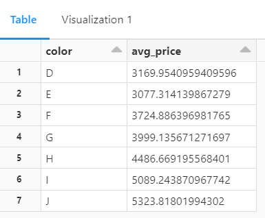
Tabular View for the Query
This SQL query above is used to retrieve the average price of diamonds based on their colors.
Let's break down the code:
SELECT color, avg(price) AS avg_price specifies the columns that will be selected in the result set. It selects the color column and calculates the average price using the avg() function. The calculated average is aliased as avg_price for easier reference in the result set.
The FROM diamonds command specifies the table from which data will be retrieved. In this case, the table is named diamonds.
GROUP BY color groups the data by the color column. The result set will contain one row for each unique color, and the average price will be calculated for each group separately.
ORDER BY color arranges the result set in ascending order based on the color column. The output will be sorted alphabetically by color.
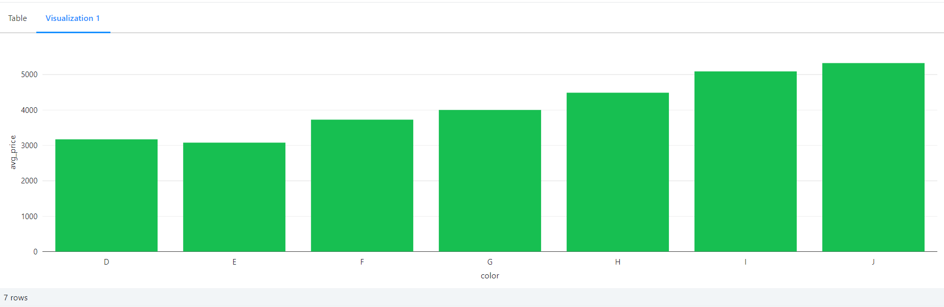
Visualized Results for the Query
Count of Diamonds by Clarity
SELECT clarity, COUNT(*) AS count
FROM diamonds
GROUP BY clarity
ORDER BY count DESC;
This SQL query above calculates the count of diamonds for each clarity level and presents the results in descending order. It selects the clarity column and uses the COUNT() function to count the number of occurrences for each clarity value.
The result set is grouped by clarity and sorted in descending order based on the count of diamonds.

Pie Chart visualization based on the above query
Average Price by Depth Range
-- This SQL query calculates the average price of diamonds grouped into depth ranges (60-62 and 62-64), and 'Other' for all other depth values, from the 'diamonds' table. The results are ordered in descending order based on the average price.

SELECT CASE
         WHEN depth BETWEEN 60 AND 62 THEN '60-62'
         WHEN depth BETWEEN 62 AND 64 THEN '62-64'
         ELSE 'Other'
       END AS depth_range,
       AVG(CAST(price AS DOUBLE)) AS avg_price
FROM diamonds
GROUP BY depth_range
ORDER BY avg_price DESC;
Here, we are calculating the average price of diamonds grouped into depth ranges. It uses a CASE statement to categorize the diamonds into three depth ranges: '60-62' for depths between 60 and 62, '62-64' for depths between 62 and 64, and 'Other' for all other depth values.
The AVG() function is then used to calculate the average price for each depth range. The result set is grouped by the depth_range column and ordered in descending order based on the average price.
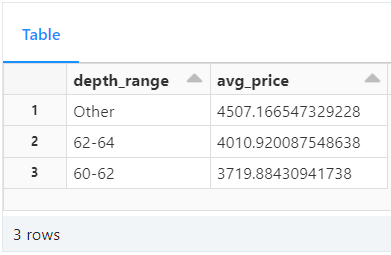
Average price based on the grouped depth range, achieved using CASE syntax
Price Distribution by Table
--  Calculate the median, first quartile (q1), and third quartile (q3) prices for each unique 'table' in the 'diamonds' table based on the 'price' column. The results are grouped by 'table' and provide valuable statistical insights into the price distribution within each category.

SELECT table,
       PERCENTILE_CONT(0.5) WITHIN GROUP (ORDER BY CAST(price AS DOUBLE)) AS median_price,
       PERCENTILE_CONT(0.25) WITHIN GROUP (ORDER BY CAST(price AS DOUBLE)) AS q1_price,
       PERCENTILE_CONT(0.75) WITHIN GROUP (ORDER BY CAST(price AS DOUBLE)) AS q3_price
FROM diamonds
GROUP BY table;
This SQL query calculates the median, first quartile (q1), and third quartile (q3) prices for each unique table value in the diamonds table. It uses the PERCENTILE_CONT() function to calculate these statistical measures.
The function is applied to the price column, which is cast as a double for accurate calculations. The result set is grouped by the table column, providing insights into the price distribution within each table category.

Casting media, Q1 and Q3 figures based on the price
Price Factor by X, Y and Z
-- Calculate the average price of diamonds grouped by their x, y, and z values from the 'diamonds' table. The results are ordered in descending order based on the average price, providing valuable insights into the average price of diamonds with different x, y, and z dimensions.

SELECT x, y, z, AVG(CAST(price AS DOUBLE)) AS avg_price
FROM diamonds
GROUP BY x, y, z
ORDER BY avg_price DESC;
This query will calculate the average price of diamonds grouped by their x, y, and z values from the diamonds table. It selects the columns x, y, z, and uses the AVG() function to calculate the average price for each combination of x, y, and z values.
The result set is then ordered in descending order based on the average price, providing insights into the average price of diamonds with different dimensions.

Visualization showing average price of diamonds grouped by their x, y, and z values from the 'diamonds' table
Add Constraints
-- This SQL code snippet alters the 'diamonds' table by dropping the existing constraint 'id_not_null' if it exists. Then, it adds a new constraint named 'id_not_null' to ensure that the column '_c0' must not contain null values, enforcing data integrity in the table.

ALTER TABLE diamonds DROP CONSTRAINT IF EXISTS id_not_null;
ALTER TABLE diamonds ADD CONSTRAINT id_not_null CHECK (_c0 is not null);
-- This command will fail as we insert a user with a null id::
INSERT INTO diamonds(_c0, carat, cut,    color,    clarity,    depth,    table,    price,    x,    y,    z) values (null, 0.22,    'Premium', 'I',    'SI2',    '60.3',    '62.1',    '334',    '3.79',    '3.75',    '2.27');
Note that this won't actually yield any output. Guess why? Because it does not stick to the NOT NULL constraint. So, whenever constraints are not fulfilled an error will be thrown. In this case, this exact error is shown:
Error in SQL statement: DeltaInvariantViolationException: CHECK constraint id_not_null (_c0 IS NOT NULL) violated by row with values:
 - _c0 : null
This SQL code snippet demonstrates the alteration of the diamonds table to enforce data integrity.
The first line of code, ALTER TABLE diamonds DROP CONSTRAINT IF EXISTS id_not_null;, checks if a constraint named id_not_null exists in the diamonds table and drops it if it does. This step ensures that any existing constraint with the same name is removed before adding a new one.
The second line of code, ALTER TABLE diamonds ADD CONSTRAINT id_not_null CHECK (_c0 is not null);, adds a new constraint named id_not_null to the diamonds table. This constraint specifies that the column _c0 must not contain null values. It ensures that whenever data is inserted or updated in this table, the '_c0' column cannot have a null value, maintaining data integrity.
However, the subsequent command, INSERT INTO diamonds(_c0, carat, cut, color, clarity, depth, table, price, x, y, z) VALUES (null, 0.22, 'Premium', 'I', 'SI2', '60.3', '62.1', '334', '3.79', '3.75', '2.27');, attempts to insert a row into the diamonds table with a null value in the _c0 column.
Since the newly added constraint prohibits null values in this column, the INSERT operation will fail, preserving the data integrity specified by the constraint.
How to Work with Dataframes
The best part is that you are not just restricted to using SQL to achieve this. Below, the same thing is done by first loading the dataset into diamonds with Python and then using pyspark library functions to do complex queries.
%python
diamonds = spark.read.csv("/databricks-datasets/Rdatasets/data-001/csv/ggplot2/diamonds.csv", header="true", inferSchema="true")
In the Databricks Delta Lake platform, the spark object represents the SparkSession, which is the entry point for interacting with Spark functionality. It provides a programming interface to work with structured and semi-structured data.
The spark.read.csv() function is used to read a CSV file into a DataFrame. In this case, it reads the diamonds.csv file from the specified path. The arguments passed to the function include:
"/databricks-datasets/Rdatasets/data-001/csv/ggplot2/diamonds.csv": This is the path to the CSV file. You can replace this with the actual path where your file is located.header="true": This specifies that the first row of the CSV file contains the column names.inferSchema="true": This instructs Spark to automatically infer the data types of the columns in the DataFrame.
Once the CSV file is read, it is stored in the diamonds variable as a DataFrame. The DataFrame represents a distributed collection of data organized into named columns. It provides various functions and methods to manipulate and analyze the data.
By reading the CSV file into a DataFrame on the Databricks Delta Lake platform, you can leverage the rich querying and processing capabilities of Spark to perform data analysis, transformations, and other operations on the diamonds data.
Manipulate the data and displays the results
The below example showcases that on the Databricks Delta Lake platform, you are not limited to using only SQL queries. You can also leverage Python and its rich ecosystem of libraries, such as PySpark, to perform complex data manipulations and analyses.
By using Python, you have access to a wide range of functions and methods provided by PySpark's DataFrame API. This allows you to perform various transformations, aggregations, calculations, and sorting operations on your data.
Whether you choose to use SQL or Python, the Databricks Delta Lake platform provides a flexible environment for data processing and analysis, enabling you to unlock valuable insights from your data.
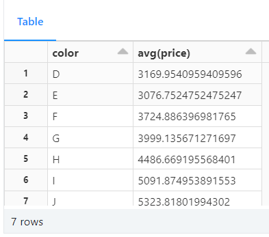
%python
from pyspark.sql.functions import avg

display(diamonds.select("color","price").groupBy("color").agg(avg("price")).sort("color"))
Firstly, the from pyspark.sql.functions import avg statement imports the avg function from the pyspark.sql.functions module. This function is used to calculate the average value of a column.
Next, the diamonds.select("color", "price").groupBy("color").agg(avg("price")).sort("color") expression performs the following operations:
diamonds.select("color", "price") selects only the color and price columns from the diamonds DataFrame.
groupBy("color") groups the data based on the color column.
agg(avg("price")) calculates the average price for each group (color). The avg("price") argument specifies that we want to calculate the average of the "price" column.
sort("color") sorts the resulting DataFrame in ascending order based on the color column.
Finally, the display() function is used to visualize the resulting DataFrame in a tabular format.
Version Control and Time Travel in Delta
Databricks Delta’s time travel capabilities simplify building data pipelines. It comes handy when auditing data changes, reproducing experiments and reports or performing database transaction rollbacks. It is also useful for disaster recovery and allows us to undo changes and shifting back to any specific version of a database.
As you write into a Delta table or directory, every operation is automatically versioned. Query a table by referring to a timestamp or a version number.
The command below returns a list of all the versions and timestamps in a table called diamonds:
DESCRIBE HISTORY diamonds;
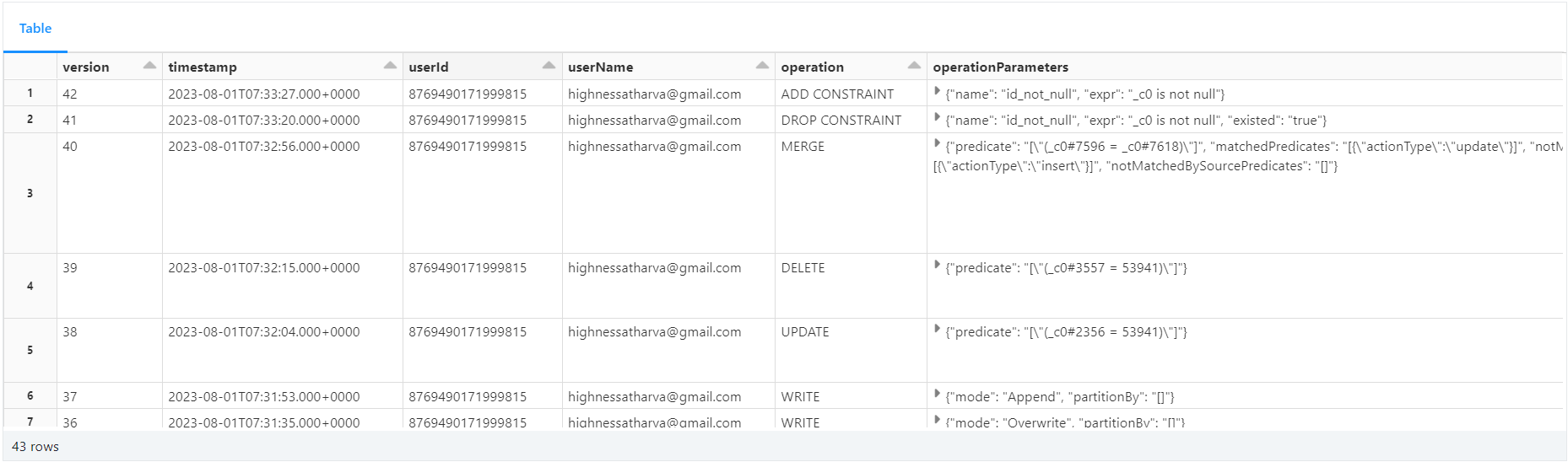
DESCRIBE HISTORY table_name returns a list of all the versions of the table along with their timestamps, operations. It also includes which user ran the query.
Restore Setup
Delta provides built-in support for backup and restore strategies to handle issues like data corruption or accidental data loss. In our scenario, we'll intentionally delete some rows from the main table to simulate such situations.
We'll then use Delta's restore capability to revert the table to a point in time before the delete operation. By doing so, we can verify if the deletion was successful or if the data was restored correctly to its previous state. This feature ensures data safety and provides an easy way to recover from undesirable changes or failures.
Here's the code:
-- Delete 10 records from the main table
DELETE FROM diamonds where `_c0`in (1,2,3,4,5,6,7,8,9,10);
SELECT COUNT(*) from diamonds;
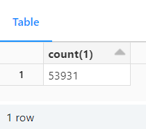
Row count after deleing 10 records from the main table
SELECT COUNT(*) FROM diamonds VERSION AS OF 19;

Row count by referencing a previous version of the table
Restoring From A Version Number
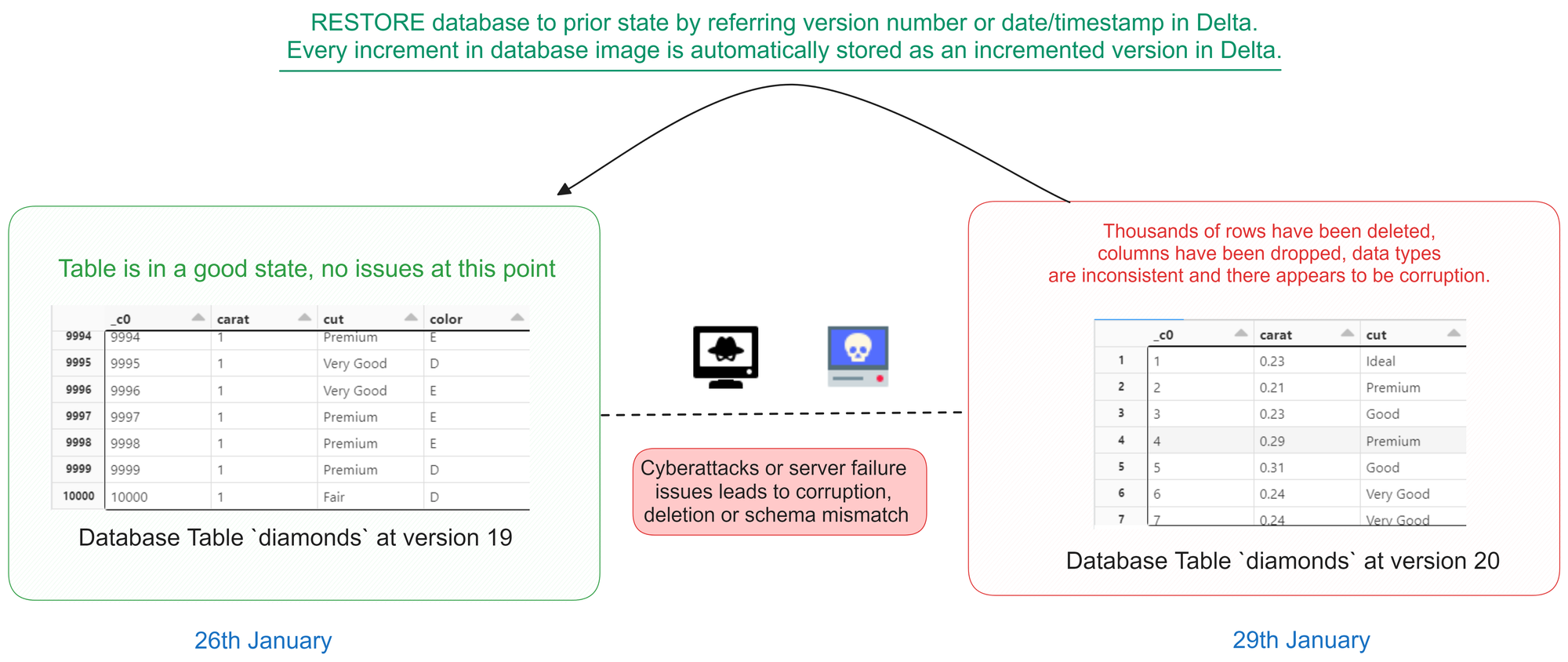
Illustration of how a Version Restore works in Databricks Notebooks
The code below restores the diamonds table to the version that existed at version number 19, using a database versioning or historical data feature. After the restoration, a SELECT statement is executed to retrieve all data from the diamonds table as it existed at version 19.
This process allows you to view the historical state of the table at that specific version, enabling data analysis or comparisons with the current version.
-- restore the state of diamonds table to that of version 19 (refer the database images in the previous cell)

RESTORE TABLE diamonds TO VERSION AS OF 19;
SELECT * from diamonds;

SELECT query running against a restored version of the database
Autogenerated Fields
Let us see how to use auto-increment in Delta with SQL. The code below demonstrates the creation of a table called test__autogen with an "autogenerated" field named id. The id column is defined as BIGINT GENERATED ALWAYS AS IDENTITY, meaning its values will be automatically generated by the database engine during the insertion process.
The id serves as an auto-incrementing primary key for the table, ensuring each new record receives a unique identifier without any manual input. This feature simplifies data insertion and guarantees the uniqueness of records within the table, enhancing database management efficiency.
This auto-incrementing feature is commonly used for primary keys, as it guarantees the uniqueness of each record in the table. It also saves developers from having to manage the generation of unique identifiers manually, providing a more streamlined and efficient workflow.
%sql
CREATE TABLE IF NOT EXISTS test__autogen (
  id BIGINT GENERATED ALWAYS AS IDENTITY ( START WITH 10000 INCREMENT BY 1 ),
  name STRING,
  surname STRING,
  email STRING,
  city STRING) ;

-- Note that we don't insert data for the id. The engine will handle that for us:
INSERT INTO test__autogen (name, surname, email, city) VALUES ('Atharva', 'Shah', 'highnessatharva@gmail.com', 'Pune, IN');
INSERT INTO test__autogen (name, surname, email, city) VALUES ('James', 'Dean', 'james@proton.mail', 'Tokyo, JP');

-- The ID is automatically generated!
SELECT * from test__autogen;
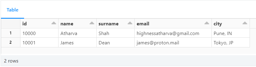
Records with an autogenerated id
Delta Table Cloning
Cloning Delta tables allows you to create a replica of an existing Delta table at a specific version. This feature is particularly valuable when you need to transfer data from a production environment to a staging environment or when archiving a specific version for regulatory purposes.
There are two types of clones available:
Deep Clone: This type of clone copies both the source table data and metadata to the clone target. In other words, it replicates the entire table, making it independent of the source.
Shallow Clone: A shallow clone only replicates the table metadata without copying the actual data files to the clone target. As a result, these clones are more cost-effective to create. However, it's crucial to note that shallow clones act as pointers to the main table. If a
VACUUMoperation is performed on the original table, it may delete the underlying files and potentially impact the shallow clone.
It's important to remember that any modifications made to either deep or shallow clones only affect the clones themselves and not the source table.
Cloning Delta tables is a powerful feature that simplifies data replication and version archiving, enhancing data management capabilities within your Delta Lake environment.
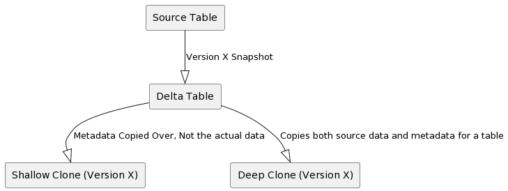
Difference between a Shallow Clone and a Deep Clone
The code below shows how to clone a table using shallow and deep clones:
-- Shallow clone (zero copy)
CREATE TABLE IF NOT EXISTS diamonds__shallow__clone
  SHALLOW CLONE diamonds
  VERSION AS OF 19;

SELECT * FROM diamonds__shallow__clone;

-- Deep clone (copy data)
CREATE TABLE IF NOT EXISTS diamonds__deep__clone
  DEEP CLONE diamonds;

SELECT * FROM diamonds__deep__clone;

Selecting records from the deep cloned table
Delta Magic Commands
There are convenient shortcuts in Databricks notebooks for managing Delta tables. They simplify common operations like displaying table metadata and running optimization.
You can use these shortcut commands to improve productivity by streamlining Delta table management tasks within a notebook environment.
%run: runs a Python file or a notebook.%sh: executes shell commands on the cluster nodes.%fs: allows you to interact with the Databricks file system.%sql: allows you to run SQL queries.%scala: switches the notebook context to Scala.%python: switches the notebook context to Python.%md: allows you to write markdown text.%r: switches the notebook context to R.%lsmagic: lists all the available magic commands.%jobs: lists all the running jobs.%config: allows you to set configuration options for the notebook.%reload: reloads the contents of a module.%pip: allows you to install Python packages.%load: loads the contents of a file into a cell.%matplotlib: sets up the matplotlib backend.%who: lists all the variables in the current scope.%env: allows you to set environment variables.
Conclusion
This in-depth handbook explored the power of Databricks, a platform that unifies analytics and data science in a single workspace. We went through Databricks Workspace, interactive analytics, and Delta Lake, emphasizing its data manipulation and analysis capabilities.
Delta, a data integrity and agility engine, supports SQL commands as well as sophisticated queries. Data frames are used to shape and display data to improve insights. Retrospection and accuracy are enabled through version control and time travel. Delta's table cloning provides innovation by permitting analytical studies into previously undiscovered territory.
Your pursuit of data excellence doesn't end here. Let's stay connected: explore more insights on my blog, consider supporting me with a cup of coffee, and join the conversation on Twitter and LinkedIn. Keep the momentum going by checking out a few of my other posts.