There's one question I always get asked regarding Data Science:

What is the best way to master Data Science? What will get me hired?

My answer remains constant: There is no alternative to working on portfolio-worthy projects.

Even after passing the TensorFlow Developer Certificate Exam, I’d say that you can only really prove your competency with projects that showcase your research, programming skills, mathematical background, and so on.

In my post how to build an effective Data Science Portfolio, I shared many project ideas and other tips to prepare an awesome portfolio. This post is dedicated to one of those ideas: building an end-to-end data science/ML project.

Agenda

This tutorial is intended to walk you through all the major steps involved in completing an and-to-end Machine Learning project. For this project, I’ve chosen a supervised learning regression problem.

Here are the major topics covered:

• Pre-requisites and Resources
• Data Collection and Problem Statement
• Exploratory Data Analysis with Pandas and NumPy
• Data Preparation using Sklearn
• Selecting and Training a few Machine Learning Models
• Cross-Validation and Hyperparameter Tuning using Sklearn
• Deploying the Final Trained Model on Heroku via a Flask App

Let’s start building…

Pre-requisites and Resources

To go through this project and tutorial, you should be familiar with Machine Learning algorithms, Python environment setup, and common ML terminologies. Here are a few resources to get you started:

• Read the first 2–3 chapters of The hundred page ML book: http://themlbook.com/wiki/doku.php
• List of Tasks for almost every Machine Learning Project — Keep referring to this list while working on this (or any other) ML project.
• You need a Python Environment set up — a virtual environment dedicated to this project.
• You should be familiar with Jupyter Notebook.

That’s it, so make sure you have an understanding of these concepts and tools and you’re ready to go!

Data Collection and Problem Statement

The first step is to get your hands on the data. But if you have access to data (as most product-based companies do), then the first step is to define the problem that you want to solve. We don’t have the data yet, so we are going to collect the data first.

We are using the Auto MPG dataset from the UCI Machine Learning Repository. Here is the link to the dataset:

• http://archive.ics.uci.edu/ml/datasets/Auto+MPG

The data concerns city-cycle fuel consumption in miles per gallon, to be predicted in terms of 3 multivalued discrete and 5 continuous attributes.

Once you have downloaded the data, move it to your project directory, activate your virtualenv, and start the Jupyter local server.

You can download the data into your project from the notebook as well using wget :

!wget "http://archive.ics.uci.edu/ml/machine-learning-databases/auto-mpg/auto-mpg.data"

The next step is to load this .data file into a pandas datagram. For that, make sure you have pandas and other general use case libraries installed. Import all the general use case libraries like so:

import numpy as np
import pandas as pd
import matplotlib.pyplot as plt
import seaborn as sns

Then read and load the file into a dataframe using the read_csv() method:

# defining the column names
cols = ['MPG','Cylinders','Displacement','Horsepower','Weight',
                'Acceleration', 'Model Year', 'Origin']
# reading the .data file using pandas
df = pd.read_csv('./auto-mpg.data', names=cols, na_values = "?",
                comment = '\t',
                sep= " ",
                skipinitialspace=True)
#making a copy of the dataframe
data = df.copy()

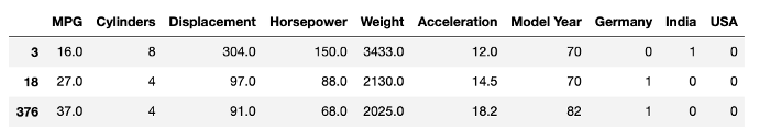
Next, look at a few rows of the dataframe and read the description of each attribute from the website. This helps you define the problem statement.

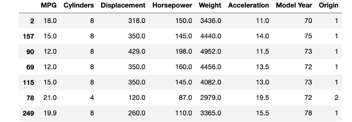
Problem Statement — The data contains the MPG (Mile Per Gallon) variable which is continuous data and tells us about the efficiency of fuel consumption of a vehicle in the 70s and 80s.

Our aim here is to predict the MPG value for a vehicle, given that we have other attributes of that vehicle.

Exploratory Data Analysis with Pandas and NumPy

For this rather simple dataset, the exploration is broken down into a series of steps:

Check for data type of columns

##checking the data info
data.info()

Check for null values.

##checking for all the null values
data.isnull().sum()

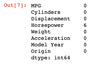
The horsepower column has 6 missing values. We’ll have to study the column a bit more.

Check for outliers in horsepower column

##summary statistics of quantitative variables
data.describe()

##looking at horsepower box plot
sns.boxplot(x=data['Horsepower'])

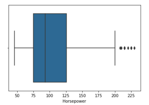
Since there are a few outliers, we can use the median of the column to impute the missing values using the pandas median() method.

##imputing the values with median
median = data['Horsepower'].median()
data['Horsepower'] = data['Horsepower'].fillna(median)
data.info()

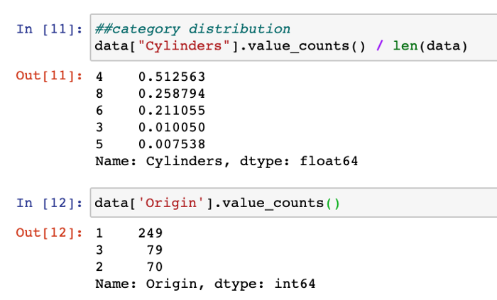
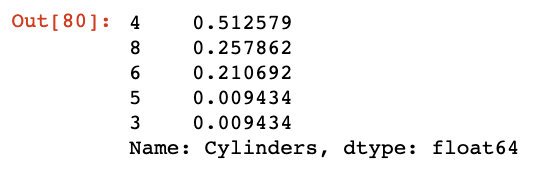
Look for the category distribution in categorical columns

##category distribution

data["Cylinders"].value_counts() / len(data)
data['Origin'].value_counts()

The 2 categorical columns are Cylinders and Origin, which only have a few categories of values. Looking at the distribution of the values among these categories will tell us how the data is distributed:

Plot for correlation

##pairplots to get an intuition of potential correlations

sns.pairplot(data[["MPG", "Cylinders", "Displacement", "Weight", "Horsepower"]], diag_kind="kde")

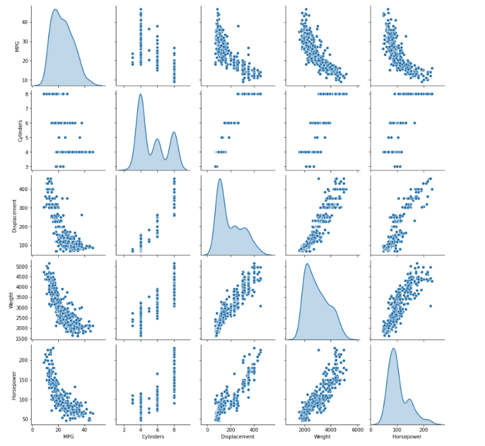
The pair plot gives you a brief overview of how each variable behaves with respect to every other variable.

For example, the MPG column (our target variable) is negatively correlated with the displacement, weight, and horsepower features.

Set aside the test data set

This is one of the first things we should do, as we want to test our final model on unseen/unbiased data.

There are many ways to split the data into training and testing sets but we want our test set to represent the overall population and not just a few specific categories. Thus, instead of using simple and common train_test_split() method from sklearn, we use stratified sampling.

Stratified Sampling — We create homogeneous subgroups called strata from the overall population and sample the right number of instances to each stratum to ensure that the test set is representative of the overall population.

In task 4, we saw how the data is distributed over each category of the Cylinder column. We’re using the Cylinder column to create the strata:

from sklearn.model_selection import StratifiedShuffleSplit

split = StratifiedShuffleSplit(n_splits=1, test_size=0.2, random_state=42)
for train_index, test_index in split.split(data, data["Cylinders"]):
    strat_train_set = data.loc[train_index]
    strat_test_set = data.loc[test_index]

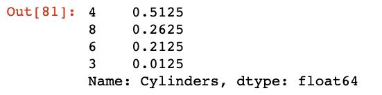
Checking for the distribution in training set:

##checking for cylinder category distribution in training set

strat_train_set['Cylinders'].value_counts() / len(strat_train_set)

Testing set:

strat_test_set["Cylinders"].value_counts() / len(strat_test_set)

You can compare these results with the output of train_test_split() to find out which one produces better splits.

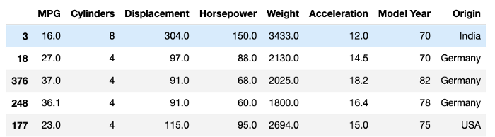
Checking the Origin Column

The Origin column about the origin of the vehicle has discrete values that look like the code of a country.

To add some complication and make it more explicit, I converted these numbers to strings:

##converting integer classes to countries in Origin 

columntrain_set['Origin'] = train_set['Origin'].map({1: 'India', 2: 'USA', 3 : 'Germany'})
train_set.sample(10)

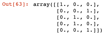
We’ll have to preprocess this categorical column by one-hot encoding these values:

##one hot encoding
train_set = pd.get_dummies(train_set, prefix='', prefix_sep='')
train_set.head()

Testing for new variables — Analyze the correlation of each variable with the target variable

## testing new variables by checking their correlation w.r.t. MPG
data['displacement_on_power'] = data['Displacement'] / data['Horsepower']
data['weight_on_cylinder'] = data['Weight'] / data['Cylinders']
data['acceleration_on_power'] = data['Acceleration'] / data['Horsepower']
data['acceleration_on_cyl'] = data['Acceleration'] / data['Cylinders']

corr_matrix = data.corr()
corr_matrix['MPG'].sort_values(ascending=False)

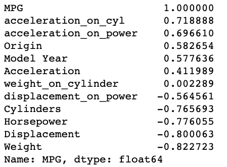
We found acceleration_on_power and acceleration_on_cyl as two new variables which turned out to be more positively correlated than the original variables.

This brings us to the end of the Exploratory Analysis. We are ready to proceed to our next step of preparing the data for Machine Learning.

Data Preparation using Sklearn

One of the most important aspects of Data Preparation is that we have to keep automating our steps in the form of functions and classes. This makes it easier for us to integrate the methods and pipelines into the main product.

Here are the major tasks to prepare the data and encapsulate functionalities:

Preprocessing Categorical Attribute — Converting the Oval

##onehotencoding the categorical values
from sklearn.preprocessing import OneHotEncoder

cat_encoder = OneHotEncoder()
data_cat_1hot = cat_encoder.fit_transform(data_cat)
data_cat_1hot   # returns a sparse matrix

data_cat_1hot.toarray()[:5]

Data Cleaning — Imputer

We’ll be using the SimpleImputer class from the impute module of the Sklearn library:

##handling missing values
from sklearn.impute import SimpleImputer

imputer = SimpleImputer(strategy="median")imputer.fit(num_data)

Attribute Addition — Adding custom transformation

In order to make changes to datasets and create new variables, sklearn offers the BaseEstimator class. Using it, we can develop new features by defining our own class.

We have created a class to add two new features as found in the EDA step above:

• acc_on_power — Acceleration divided by Horsepower
• acc_on_cyl — Acceleration divided by the number of Cylinders

from sklearn.base import BaseEstimator, TransformerMixin

acc_ix, hpower_ix, cyl_ix = 4, 2, 0

##custom class inheriting the BaseEstimator and TransformerMixin
class CustomAttrAdder(BaseEstimator, TransformerMixin):
    def __init__(self, acc_on_power=True):
        self.acc_on_power = acc_on_power  # new optional variable
    def fit(self, X, y=None):
        return self  # nothing else to do
    def transform(self, X):
        acc_on_cyl = X[:, acc_ix] / X[:, cyl_ix] # required new variable
        if self.acc_on_power:
            acc_on_power = X[:, acc_ix] / X[:, hpower_ix]
            return np.c_[X, acc_on_power, acc_on_cyl] # returns a 2D array
        
        return np.c_[X, acc_on_cyl]
    
attr_adder = CustomAttrAdder(acc_on_power=True)
data_tr_extra_attrs = attr_adder.transform(data_tr.values)
data_tr_extra_attrs[0]

Setting up Data Transformation Pipeline for numerical and categorical attributes

As I said, we want to automate as much as possible. Sklearn offers a great number of classes and methods to develop such automated pipelines of data transformations.

The major transformations are to be performed on numerical columns, so let’s create the numerical pipeline using the Pipeline class:

def num_pipeline_transformer(data):
    '''
    Function to process numerical transformations
    Argument:
        data: original dataframe 
    Returns:
        num_attrs: numerical dataframe
        num_pipeline: numerical pipeline object
        
    '''
    numerics = ['float64', 'int64']

    num_attrs = data.select_dtypes(include=numerics)

    num_pipeline = Pipeline([
        ('imputer', SimpleImputer(strategy="median")),
        ('attrs_adder', CustomAttrAdder()),
        ('std_scaler', StandardScaler()),
        ])
    return num_attrs, num_pipeline

In the above code snippet, we have cascaded a set of transformations:

• Imputing Missing Values — using the SimpleImputer class discussed above.
• Custom Attribute Addition— using the custom attribute class defined above.
• Standard Scaling of each Attribute — always a good practice to scale the values before feeding them to the ML model, using the standardScaler class.

Combined Pipeline for both Numerical and Categorical columns

We have the numerical transformation ready. The only categorical column we have is Origin for which we need to one-hot encode the values.

Here’s how we can use the ColumnTransformer class to capture both of these tasks in one go.

def pipeline_transformer(data):
    '''
    Complete transformation pipeline for both
    nuerical and categorical data.
    
    Argument:
        data: original dataframe 
    Returns:
        prepared_data: transformed data, ready to use
    '''
    cat_attrs = ["Origin"]
    num_attrs, num_pipeline = num_pipeline_transformer(data)
    full_pipeline = ColumnTransformer([
        ("num", num_pipeline, list(num_attrs)),
        ("cat", OneHotEncoder(), cat_attrs),
        ])
    prepared_data = full_pipeline.fit_transform(data)
    return prepared_data

To the instance, provide the numerical pipeline object created from the function defined above. Then call the OneHotEncoder() class to process the Origin column.

Final Automation

With these classes and functions defined, we now have to integrate them into a single flow which is going to be simply two function calls.

1. Preprocessing the Origin Column to convert integers to Country names:

##preprocess the Origin column in data
def preprocess_origin_cols(df):
    df["Origin"] = df["Origin"].map({1: "India", 2: "USA", 3: "Germany"})    
    return df

2.  Calling the final pipeline_transformer function defined above:

##from raw data to processed data in 2 steps

preprocessed_df = preprocess_origin_cols(data)
prepared_data = pipeline_transformer(preprocessed_df)prepared_data

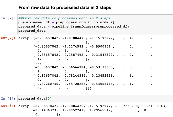
Voilà, your data is ready to use in just two steps!

The next step is to start training our ML models.

Selecting and Training Machine Learning Models

Since this is a regression problem, I chose to train the following models:

1. Linear Regression
2. Decision Tree Regressor
3. Random Forest Regressor
4. SVM Regressor

I’ll explain the flow for Linear Regression and then you can follow the same for all the others.

It’s a simple 4-step process:

1. Create an instance of the model class.
2. Train the model using the fit() method.
3. Make predictions by first passing the data through pipeline transformer.
4. Evaluating the model using Root Mean Squared Error (typical performance metric for regression problems)

from sklearn.linear_model import LinearRegression

lin_reg = LinearRegression()
lin_reg.fit(prepared_data, data_labels)

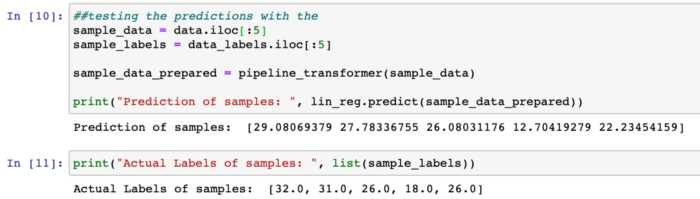
##testing the predictions with first 5 rows
sample_data = data.iloc[:5]
sample_labels = data_labels.iloc[:5]
sample_data_prepared = pipeline_transformer(sample_data)

print("Prediction of samples: ", lin_reg.predict(sample_data_prepared))

Evaluating model:

from sklearn.metrics import mean_squared_error

mpg_predictions = lin_reg.predict(prepared_data)
lin_mse = mean_squared_error(data_labels, mpg_predictions)
lin_rmse = np.sqrt(lin_mse)lin_rmse

RMSE for Linear regression: 2.95904

Cross-Validation and Hyperparameter Tuning using Sklearn

Now, if you perform the same for Decision Tree, you’ll see that you have achieved a 0.0 RMSE value which is not possible – there is no “perfect” Machine Learning Model (we’ve not reached that point yet).

Problem: we are testing our model on the same data we trained on, which is a problem. Now, we can’t use the test data yet until we finalize our best model that is ready to go into production.

Solution: Cross-Validation

Scikit-Learn’s K-fold cross-validation feature randomly splits the training set into K distinct subsets called folds. Then it trains and evaluates the model K times, picking a different fold for evaluation every time and training on the other K-1 folds.

The result is an array containing the K evaluation scores. Here’s how I did for 10 folds:

from sklearn.model_selection import cross_val_score

scores = cross_val_score(tree_reg, 
                         prepared_data, 
                         data_labels, 
                         scoring="neg_mean_squared_error", 
                         cv = 10)
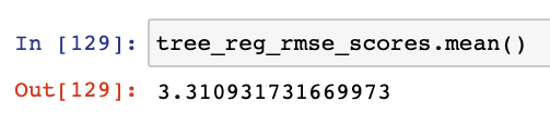
tree_reg_rmse_scores = np.sqrt(-scores)

The scoring method gives you negative values to denote errors. So while calculating the square root, we have to add negation explicitly.

For Decision Tree, here is the list of all scores:

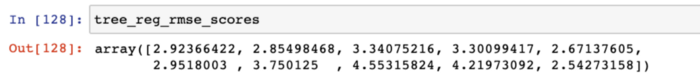
Take the average of these scores:

Fine-Tuning Hyperparameters

After testing all the models, you’ll find that RandomForestRegressor has performed the best but it still needs to be fine-tuned.

A model is like a radio station with a lot of knobs to handle and tune. Now, you can either tune all these knobs manually or provide a range of values/combinations that you want to test.

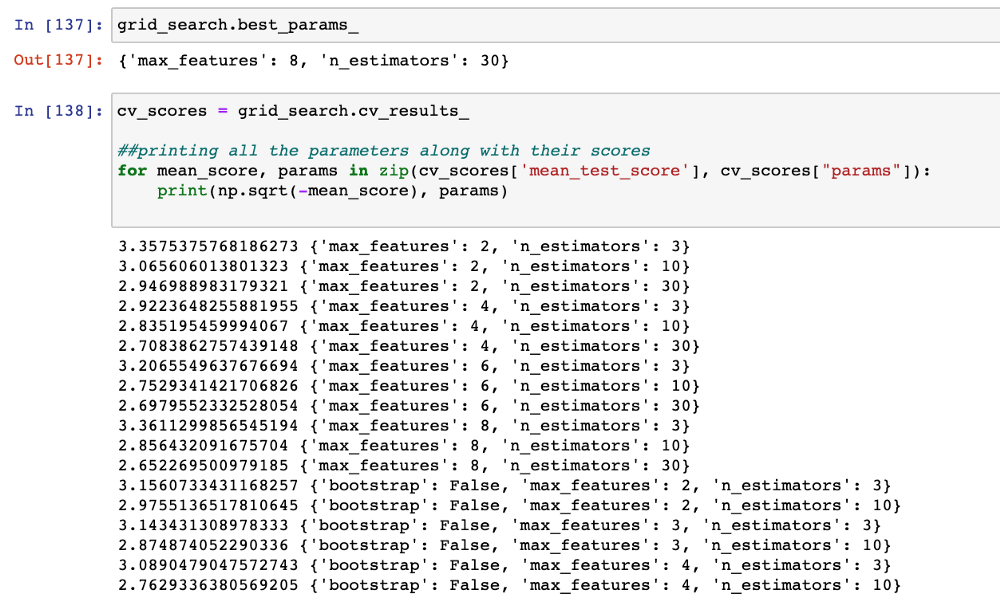
We use GridSearchCV to find out the best combination of hyperparameters for the RandomForest model:

from sklearn.model_selection import GridSearchCV

param_grid = [
    {'n_estimators': [3, 10, 30], 'max_features': [2, 4, 6, 8]},
    {'bootstrap': [False], 'n_estimators': [3, 10], 'max_features': [2, 3, 4]},
  ]

forest_reg = RandomForestRegressor()

grid_search = GridSearchCV(forest_reg, param_grid,
                           scoring='neg_mean_squared_error',
                           return_train_score=True,
                           cv=10,
                          )

grid_search.fit(prepared_data, data_labels)

GridSearchCV requires you to pass the parameter grid. This is a python dictionary with parameter names as keys mapped with the list of values you want to test for that param.

We can pass the model, scoring method, and cross-validation folds to it.

Train the model and it returns the best parameters and results for each combination of parameters:

Check Feature Importance

We can also check the feature importance by enlisting the features and zipping them up with the best_estimator’s feature importance attribute as follows:

# feature importances
feature_importances = grid_search.best_estimator_.feature_importances_

extra_attrs = ["acc_on_power", "acc_on_cyl"]
numerics = ['float64', 'int64']
num_attrs = list(data.select_dtypes(include=numerics))

attrs = num_attrs + extra_attrs
sorted(zip(attrs, feature_importances), reverse=True)

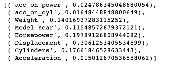
We see that acc_on_power, which is the derived feature, has turned out to be the most important feature.

You might want to keep iterating a few times before finalizing the best configuration.

The model is now ready with the best configuration.

Evaluate the Entire System

It’s time to evaluate this entire system:

##capturing the best configuration
final_model = grid_search.best_estimator_

##segregating the target variable from test set
X_test = strat_test_set.drop("MPG", axis=1)
y_test = strat_test_set["MPG"].copy()

##preprocessing the test data origin column
X_test_preprocessed = preprocess_origin_cols(X_test)

##preparing the data with final transformation
X_test_prepared = pipeline_transformer(X_test_preprocessed)

##making final predictions
final_predictions = final_model.predict(X_test_prepared)
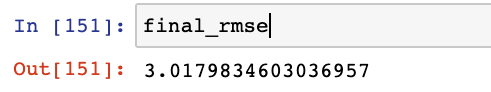
final_mse = mean_squared_error(y_test, final_predictions)
final_rmse = np.sqrt(final_mse)

If you want to look at my complete project, here is the GitHub repository:

With that, you have your final model ready to go into production.

For deployment, we save our model into a file using the pickle model and develop a Flask web service to be deployed in Heroku. Let's see how that works now.

What do you need to deploy the application?

In order to deploy any trained model, you need the following:

• A trained model ready to deploy — save the model into a file to be further loaded and used by the web service.
• A web service — that gives a purpose for your model to be used in practice. For our fuel consumption model, it can be using the vehicle configuration to predict its efficiency. We’ll use Flask to develop this service.
• A cloud service provider — you need special cloud servers to deploy the application. For simplicity, we are going to use Heroku for this (I'll cover AWS and GCP in other articles).

Let’s get started by looking at each of these processes one by one.

Saving the Trained Model

Once you’re confident enough to take your trained and tested model into the production-ready environment, the first step is to save it into a .h5 or .bin file using a library like pickle .

Make sure you have pickle installed in your environment.

Next, let’s import the module and dump the model into a .bin file:

import pickle

##dump the model into a file
with open("model.bin", 'wb') as f_out:
    pickle.dump(final_model, f_out) # write final_model in .bin file
    f_out.close()  # close the file 

This will save your model in your present working directory unless you specify some other path.

It’s time to test if we are able to use this file to load our model and make predictions. We are going to use the same vehicle config as we defined above:

##vehicle config
vehicle_config = {
    'Cylinders': [4, 6, 8],
    'Displacement': [155.0, 160.0, 165.5],
    'Horsepower': [93.0, 130.0, 98.0],
    'Weight': [2500.0, 3150.0, 2600.0],
    'Acceleration': [15.0, 14.0, 16.0],
    'Model Year': [81, 80, 78],
    'Origin': [3, 2, 1]
}

Let’s load the model from the file:

##loading the model from the saved file
with open('model.bin', 'rb') as f_in:
    model = pickle.load(f_in)

Make predictions on the vehicle_config:

##defined in prev_blog
predict_mpg(vehicle_config, model)


##output: array([34.83333333, 18.50666667, 20.56333333])

The output is the same as we predicted earlier using final_model.

Developing a web service

The next step is to package this model into a web service that, when given the data through a POST request, returns the MPG (Miles per Gallon) predictions as a response.

I am using the Flask web framework, a commonly used lightweight framework for developing web services in Python. In my opinion, it is probably the easiest way to implement a web service.

Flask gets you started with very little code and you don’t need to worry about the complexity of handling with HTTP requests and responses.

Here are the steps:

• Create a new directory for your flask application.
• Set up a dedicated environment with dependencies installed using pip.
• Install the following packages:

pandas
numpy
sklearn
flask
gunicorn
seaborn

The next step is to activate this environment and start developing a simple endpoint to test the application:

Create a new file, main.py and import the flask module:

from flask import Flask

Create a Flask app by instantiating the Flask class:

##creating a flask app and naming it "app"
app = Flask('app')

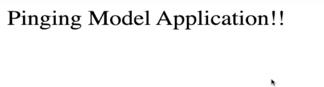
Create a route and a function corresponding to it that will return a simple string:

@app.route('/test', methods=['GET'])
def test():
    return 'Pinging Model Application!!'

The above code makes use of decorators — an advanced Python feature. You can read more about decorators here.

We don’t need a deep understanding of decorators, just that adding a decorator @app.route on top of the test() function assigns that web service address to that function.

Now, to run the application we need this last piece of code:

if __name__ == ‘__main__’:
    app.run(debug=True, host=’0.0.0.0', port=9696)

The run method starts our flask application service. The 3 parameters specify:

• debug=True — restarts the application automatically when it encounters any change in the code
• host=’0.0.0.0' — makes the web service public
• port=9696 — the port that we use to access the application

Now, in your terminal run the main.py:

python main.py

Opening the URL http://0.0.0.0:9696/test in your browser will print the response string on the webpage:

With the application now running, let’s run the model.

Create a new directory model_files to store all the model-related code.

In this directory, create a ml_model.py file which will contain the data preparation code and the predict function we wrote here.

Copy and paste the libraries you imported earlier in the article and the preprocessing/transformation functions. The file should look like this:

import numpy as np
import pandas as pd
import matplotlib.pyplot as plt
import seaborn as sns

from sklearn.model_selection import train_test_split
from sklearn.preprocessing import OneHotEncoder
from sklearn.base import BaseEstimator, TransformerMixin
from sklearn.impute import SimpleImputer

from sklearn.pipeline import Pipeline
from sklearn.preprocessing import StandardScaler
from sklearn.compose import ColumnTransformer


##functions


def preprocess_origin_cols(df):
    df["Origin"] = df["Origin"].map({1: "India", 2: "USA", 3: "Germany"})
    return df


acc_ix, hpower_ix, cyl_ix = 3, 5, 1

class CustomAttrAdder(BaseEstimator, TransformerMixin):
    def __init__(self, acc_on_power=True): # no *args or **kargs
        self.acc_on_power = acc_on_power
    def fit(self, X, y=None):
        return self  # nothing else to do
    def transform(self, X):
        acc_on_cyl = X[:, acc_ix] / X[:, cyl_ix]
        if self.acc_on_power:
            acc_on_power = X[:, acc_ix] / X[:, hpower_ix]
            return np.c_[X, acc_on_power, acc_on_cyl]
        
        return np.c_[X, acc_on_cyl]


def num_pipeline_transformer(data):
    numerics = ['float64', 'int64']

    num_attrs = data.select_dtypes(include=numerics)

    num_pipeline = Pipeline([
        ('imputer', SimpleImputer(strategy="median")),
        ('attrs_adder', CustomAttrAdder()),
        ('std_scaler', StandardScaler()),
        ])
    return num_attrs, num_pipeline


def pipeline_transformer(data):
    
    cat_attrs = ["Origin"]
    num_attrs, num_pipeline = num_pipeline_transformer(data)
    
    full_pipeline = ColumnTransformer([
        ("num", num_pipeline, list(num_attrs)),
        ("cat", OneHotEncoder(), cat_attrs),
        ])
    full_pipeline.fit_transform(data)
    return full_pipeline    


def predict_mpg(config, model):
    
    if type(config) == dict:
        df = pd.DataFrame(config)
    else:
        df = config
    
    preproc_df = preprocess_origin_cols(df)
    print(preproc_df)
    pipeline = pipeline_transformer(preproc_df)
    prepared_df = pipeline.transform(preproc_df)
    print(len(prepared_df[0]))
    y_pred = model.predict(prepared_df)
    return y_pred
    

In the same directory add your saved model.bin file as well.

Now, in the main.py we are going to import the predict_mpg function to make predictions. But to do that we are required to create an empty __init__.py file to tell Python that the directory is a package.

Your directory should have this tree:

Next up, define the predict/ route that will accept the vehicle_config from an HTTP POST request and return the predictions using the model and predict_mpg() method.

In your main.py, first import:

import pickle
from flask import Flask, request, jsonify
from model_files.ml_model import predict_mpg

Then add the predict route and the corresponding function:

@app.route('/predict', methods=['POST'])
def predict():
    vehicle = request.get_json()
    print(vehicle)
    with open('./model_files/model.bin', 'rb') as f_in:
        model = pickle.load(f_in)
        f_in.close()
    predictions = predict_mpg(vehicle, model)

    result = {
        'mpg_prediction': list(predictions)
    }
    return jsonify(result)

Here, we’ll only be accepting POST request for our function and thus we have methods=[‘POST’] in the decorator.

• First, we capture the data( vehicle_config) from our request using the get_json() method and store it in the variable vehicle.
• Then we load the trained model into the model variable from the file we have in the model_files folder.
• Now, we make the predictions by calling the predict_mpg function and passing the vehicle and model.
• We create a JSON response of this array returned in the predictions variable and return this JSON as the method response.

We can test this route using Postman or the requests package and then start the server running the main.py. Then in your notebook, add this code to send a POST request with the vehicle_config:

import requests

url = “http://localhost:9696/predict"
r = requests.post(url, json = vehicle_config)
r.text.strip()

##output: '{"mpg_predictions":[34.60333333333333,19.32333333333333,14.893333333333333]}'

Great! Now, comes the last part: this same functionality should work when deployed on a remote server.

Deploying the application on Heroku

To deploy this flask application on Heroku, you need to follow these very simple steps:

1. Create a Procfile in the main directory — this contains the command to get the run the application on the server.
2. Add the following in your Procfile:

web: gunicorn wsgi:app

We are using gunicorn (installed earlier) to deploy the application:

Gunicorn is a pure-Python HTTP server for WSGI applications. It allows you to run any Python application concurrently by running multiple Python processes within a single dyno. It provides a perfect balance of performance, flexibility, and configuration simplicity.

Now, create a wsgi.py file and add:

##importing the app from main file
from main import app

if __name__ == “__main__”: 
    app.run()

Make sure you delete the run code from the main.py .

Write all the python dependencies into requirements.txt.

You can use pip freeze > requirements.txt or simply put the above-mentioned list of packages + any other package that your application is using.

Now, using the terminal,

• initialize an empty git repository,
• add the files to the staging area,
• and commit files to the local repository:

$ git init 
$ git add .
$ git commit -m "Initial Commit"

Next, create a Heroku account if you haven’t already. Then login to the Heroku CLI:

heroku login

Approve the login from the browser as the page pops up.

Now create a flask app:

heroku create <name of your app>

I named it mpg-flask-app. It will create a flask app and will give us a URL on which the app will be deployed.

Finally, push all your code to Heroku remote:

$ git push heroku master

And Voilà! Your web service is now deployed on https://mpg-flask-app.herokuapp.com/predict.

Again, test the endpoint using the request package by sending the same vehicle config:

With that, you have all the major skills you need to start building more complex ML applications.

You can refer to my GitHub repository for this project.

And you can develop this entire project along with me:

Next Steps

This was still a simple project. For the next steps, I’d recommend you take up a more complex dataset – maybe pick up a classification problem and repeat these tasks until deployment.

Check out Data Science with Harshit — My YouTube Channel

Here is the complete tutorial (in playlist form) on my YouTube channel where you can follow me while working on this project.

With this channel, I plan to roll out a couple of series covering the entire data science space. Here is why you should be subscribing to the channel:

• These series would cover all the required/demanded quality tutorials on each of the topics and subtopics like Python fundamentals for Data Science.
• Explained Mathematics and derivations of why we do what we do in ML and Deep Learning.
• Podcasts with Data Scientists and Engineers at Google, Microsoft, Amazon, etc, and CEOs of big data-driven companies.
• Projects and instructions to implement the topics learned so far. Learn about new certifications, Bootcamp, and resources to crack those certifications like this TensorFlow Developer Certificate Exam by Google.

If this tutorial was helpful, you should check out my data science and machine learning courses on Wiplane Academy. They are comprehensive yet compact and helps you build a solid foundation of work to showcase.