They say data is the new oil, but we don't use oil directly from its source. It has to be processed and cleaned before we use it for different purposes.

The same applies to data, we don't use it directly from its source. It also has to be processed.

imageonline-co-merged-image — Oil industry

This may be a challenge for beginners in Machine Learning and Data science because data comes from different sources with different data types. Therefore you can not apply the same method of cleaning and processing to different types of data.

"Information can be extracted from data just as energy can be extracted from oil."- Adeola Adesina

You have to learn and apply methods depending on the data you have. Then you can get insight from it or use it for training in machine learning or deep learning algorithms.

After reading this article, you will know:

What is feature engineering and feature selection.
Different methods to handle missing data in your dataset.
Different methods to handle continuous features.
Different methods to handle categorical features.
Different methods for feature selection.

Let's get started.🚀

What is Feature Engineering?

Feature engineering refers to a process of selecting and transforming variables/features in your dataset when creating a predictive model using machine learning.

Therefore you have to extract the features from the raw dataset you have collected before training your data in machine learning algorithms.
Otherwise, it will be hard to gain good insights in your data.

Torture the data, and it will confess to anything. — Ronald Coase

Feature engineering has two goals:

Preparing the proper input dataset, compatible with the machine learning algorithm requirements.
Improving the performance of machine learning models.

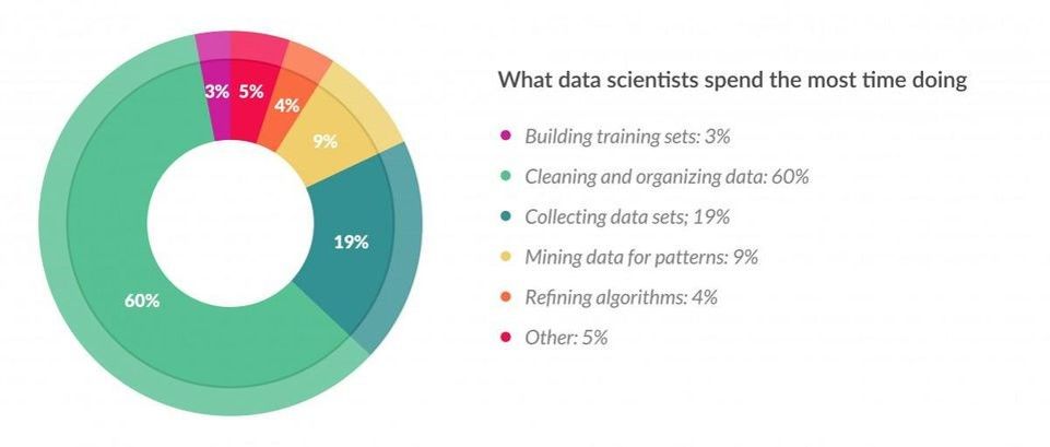
According to a survey of 80 Data Scientists conducted by CrowdFlower, Data Scientists spend 60% of their time cleaning and organizing data. This is why having skills in feature engineering and selection is very important.

“ At the end of the day, some machine learning projects succeed, and some fail. What makes the difference? Easily the most important factor is the features used. ” — Prof. Pedro Domingos from the University of Washington

You can read his paper from the following link: "A Few Useful Things to Know About Machine Learning".

Now that you know why you need to learn different techniques for feature engineering, let's start by learning different methods to handle missing data.

How to Handle Missing Data

Handling missing data is very important as many machine learning algorithms do not support data with missing values. If you have missing values in the dataset, it can cause errors and poor performance with some machine learning algorithms.

Here is the list of common missing values you can find in your dataset.

N/A
null
Empty
?
none
empty
-
NaN

Let's learn different methods to solve the problem of missing data.

Variable Deletion

Variable deletion involves dropping variables (columns) with missing values on a case-by-case basis. This method makes sense when there are a lot of missing values in a variable and if the variable is of relatively less importance.

The only case that it may worth deleting a variable is when its missing values are more than 60% of the observations.

# import packages
import numpy as np 
import pandas as pd 

# read dataset 
data = pd.read_csv('path/to/data')

#set threshold
threshold = 0.7

# dropping columns with missing value rate higher than threshold
data = data[data.columns[data.isnull().mean() < threshold]]

In the code snippet above, you can see how I use NumPy and pandas to load the dataset and set a threshold to 0.7. This means any column that has missing values of more than 70% of the observations will be dropped from the dataset.

I recommend you set your threshold value depending on the size of your dataset.

Mean or Median Imputation

Another common technique is to use the mean or median of the non-missing observations. This strategy can be applied to a feature that has numeric data.

# filling missing values with medians of the columns
data = data.fillna(data.median())

In the example above, we use the median method to fill missing values in the dataset.

Most Common Value

This method is replacing the missing values with the maximum occurred value in a column/feature. This is a good option for handling categorical columns/features.

# filling missing values with medians of the columns
data['column_name'].fillna(data['column_name'].value_counts().idxmax(). inplace=True)

Here we use the value_counts() method from pandas to count the occurrence of each unique value in the column and then fill the missing value with the most common value.

How to Handle Continuous Features

Continuous features in the dataset have a different range of values. Common examples of continuous features are age, salary, prices, and heights.

It is very important to handle continuous features in your dataset before you train machine learning algorithms. If you train your model with a different range of values, the model will not perform well.

What do I mean when I say a different range of values? Let's say you have a dataset that has two continuous features, age and salary. The range of age will be different from range of salary, and that can cause problems.

Here are some common methods to handle continuous features:

Min-Max Normalization

For each value in a feature, Min-Max normalization subtracts the minimum value in the feature and then divides by its range. The range is the difference between the original maximum and the original minimum.

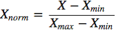
Finally, it scales all values in a fixed range between 0 and 1.

You can use the MinMaxScaler method from Scikit-learn that transforms features by scaling each feature to a given range:

from sklearn.preprocessing import MinMaxScaler
import numpy as np

# 4 samples/observations and 2 variables/features
data = np.array([[4, 6], [11, 34], [10, 17], [1, 5]])

# create scaler method
scaler = MinMaxScaler(feature_range=(0,1))

# fit and transform the data
scaled_data = scaler.fit_transform(data)

print(scaled_data)

# [[0.3        0.03448276]
#  [1.         1.        ] 
#  [0.9        0.4137931 ] 
#  [0.         0.        ]]

As you can see, our data has been transformed and the range is between 0 and 1.

Standardization

The Standardization ensures that each feature has a mean of 0 and a standard deviation of 1, bringing all features to the same magnitude.

If the standard deviation of features is different, their range would also differ.

x = observation, μ = mean , σ = standard deviation

You can use the StandardScaler method from Scikit-learn to standardize features by removing the mean and scaling to a standard deviation of 1:

from sklearn.preprocessing import StandardScaler
import numpy as np

# 4 samples/observations and 2 variables/features
data = np.array([[4, 1], [11, 1], [10, 4], [1, 11]])

# create scaler method 
scaler = StandardScaler()

# fit and transform the data
scaled_data = scaler.fit_transform(data)

print(scaled_data)

# [[-0.60192927 -0.79558708]
#  [ 1.08347268 -0.79558708] 
#  [ 0.84270097 -0.06119901] 
#  [-1.32424438  1.65237317]]

Let's verify that the mean of each feature (column) is 0:

print(scaled_data.mean(axis=0))

[0. 0.]

And that the standard deviation of each feature (column) is 1:

print(scaled_data.std(axis=0))

[1. 1.]

How to Handle Categorical Features

Categorical features represent types of data that may be divided into groups. For example, genders and educational levels.

Any non-numerical values need to be converted to integers or floats to be utilized in most machine learning libraries.

Common methods to handle categorical features are:

Label Encoding

Label encoding is simply converting each categorical value in a column to a number.

It is recommended to use label encoding to convert them into binary variables.

In the following example, you will learn how to use LableEncoder from Scikit-learn to transform categorical values into binary:

# import packages
import numpy as np 
import pandas as pd 
from sklearn.preprocessing import LabelEncoder

# intialise data of lists.
data = {'Gender':['male', 'female', 'female', 'male','male'],
        'Country':['Tanzania','Kenya', 'Tanzania', 'Tanzania','Kenya']}
  
# Create DataFrame
data = pd.DataFrame(data)


# create label encoder object
le = LabelEncoder()
  
data['Gender']= le.fit_transform(data['Gender'])
data['Country']= le.fit_transform(data['Country'])

print(data)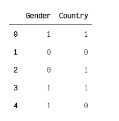

One-hot-encoding

By far the most common way to represent categorical variables is using the one-hot encoding, or one-out-of-N encoding methods, also known as dummy variables.

The idea behind dummy variables is to replace a categorical variable with one or more new features that can have the values 0 and 1.

In the following example, we will use encoders from the Scikit-learn library. LabelEncoder will help us to create an integer encoding of labels from our data and OneHotEncoder will create a one-hot encoding of integer encoded values.

# import packages 
import numpy as np 
from sklearn.preprocessing import OneHotEncoder, LabelEncoder


# define example
data = np.array(['cold', 'cold', 'warm', 'cold', 'hot', 'hot', 'warm', 'cold', 'warm', 'hot'])

# integer encode
label_encoder = LabelEncoder()

#fit and transform the data
integer_encoded = label_encoder.fit_transform(data)
print(integer_encoded)

# one-hot encode
onehot_encoder = OneHotEncoder(sparse=False)

#reshape the data
integer_encoded = integer_encoded.reshape(len(integer_encoded), 1)

#fit and transform the data
onehot_encoded = onehot_encoder.fit_transform(integer_encoded)

print(onehot_encoded)

This is the ouput of integer_encoded by LabelEncoder method:

[0 0 2 0 1 1 2 0 2 1]

And this is the output of onehot_encoded by OneHotEncoder method:

[[1. 0. 0.] 
 [1. 0. 0.] 
 [0. 0. 1.] 
 [1. 0. 0.] 
 [0. 1. 0.] 
 [0. 1. 0.] 
 [0. 0. 1.] 
 [1. 0. 0.] 
 [0. 0. 1.] 
 [0. 1. 0.]]

What is Feature Selection?

Feature selection is the process where you automatically or manually select the features that contribute the most to your prediction variable or output.

Having irrelevant features in your data can decrease the accuracy of the machine learning models.

The top reasons to use feature selection are:

It enables the machine learning algorithm to train faster.
It reduces the complexity of a model and makes it easier to interpret.
It improves the accuracy of a model if the right subset is chosen.
It reduces overfitting.

“I prepared a model by selecting all the features and I got an accuracy of around 65% which is not pretty good for a predictive model and after doing some feature selection and feature engineering without doing any logical changes in my model code my accuracy jumped to 81% which is quite impressive”- By Raheel Shaikh

Common methods for feature selection are:

Univariate Selection

Statistical tests can help to select independent features that have the strongest relationship with the target feature in your dataset. For example, the chi-squared test.

The Scikit-learn library provides the SelectKBest class that can be used with a suite of different statistical tests to select a specific number of features.

In the following example we use the SelectKBest class with the chi-squired test to find best feature for the Iris dataset:

# Load packages
from sklearn.datasets import load_iris
from sklearn.feature_selection import SelectKBest
from sklearn.feature_selection import chi2
  
# Load iris data
iris_dataset = load_iris()
  
# Create features and target
X = iris_dataset.data
y = iris_dataset.target
  
# Convert to categorical data by converting data to integers
X = X.astype(int)
  
# Two features with highest chi-squared statistics are selected
chi2_features = SelectKBest(chi2, k = 2)
X_kbest_features = chi2_features.fit_transform(X, y)
  
# Reduced features
print('Original feature number:', X.shape[1])
print('Reduced feature number:', X_kbest_features.shape[1])

Original feature number: 4
Reduced feature number: 2

As you can see chi-squared test helps us to select two important independent features out of the original 4 that have the strongest relationship with the target feature.

You can learn more about chi-squared test here: "A Gentle Introduction to the Chi-Squared Test for Machine Learning".

Feature Importance

Feature importance gives you a score for each feature of your data. The higher the score, the more important or relevant that feature is to your target feature.

Feature importance is an inbuilt class that comes with tree-based classifiers such as:

Random Forest Classifiers
Extra Tree Classifiers

In the following example, we will train the extra tree classifier into the iris dataset and use the inbuilt class .feature_importances_ to compute the importance of each feature:

# Load libraries
from sklearn.datasets import load_iris
import matplotlib.pyplot as plt
from sklearn.ensemble import ExtraTreesClassifier

# Load iris data
iris_dataset = load_iris()
  
# Create features and target
X = iris_dataset.data
y = iris_dataset.target
  
# Convert to categorical data by converting data to integers
X = X.astype(int)
 
 # Building the model
extra_tree_forest = ExtraTreesClassifier(n_estimators = 5,
                                        criterion ='entropy', max_features = 2)
  
# Training the model
extra_tree_forest.fit(X, y)
  
# Computing the importance of each feature
feature_importance = extra_tree_forest.feature_importances_
  
# Normalizing the individual importances
feature_importance_normalized = np.std([tree.feature_importances_ for tree in 
                                        extra_tree_forest.estimators_],
                                        axis = 0)

# Plotting a Bar Graph to compare the models
plt.bar(iris_dataset.feature_names, feature_importance_normalized)
plt.xlabel('Feature Labels')
plt.ylabel('Feature Importances')
plt.title('Comparison of different Feature Importances')
plt.show()

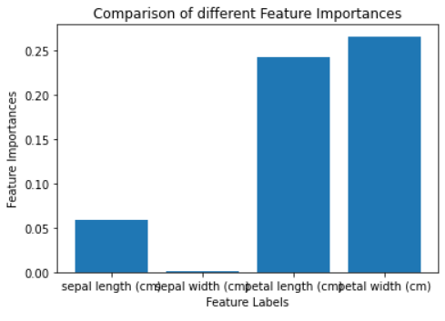
The above graph shows that the most important features are petal length (cm) and petal width (cm), and that the least important feature is sepal width (cms). This means you can use the most important features to train your model and get best performance.

Correlation Matrix Heatmap

Correlation shows how the features are related to each other or the target feature.

Correlation can be positive (an increase in one value of the feature increases the value of the target variable) or negative (an increase in one value of the feature decreases the value of the target variable).

In the following example, we will use the Boston house prices dataset from the Scikit-learn library and the corr() method from pandas to find the pairwise correlation of all features in the dataframe:

# Load libraries
from sklearn.datasets import load_boston
import matplotlib.pyplot as plt
import seaborn as sns


# load boston data
boston_dataset = load_boston()

# create a daframe for boston data
boston = pd.DataFrame(boston_dataset.data, columns=boston_dataset.feature_names)
  
# Convert to categorical data by converting data to integers
#X = X.astype(int)
 
#ploting the heatmap for correlation
ax = sns.heatmap(boston.corr().round(2), annot=True)

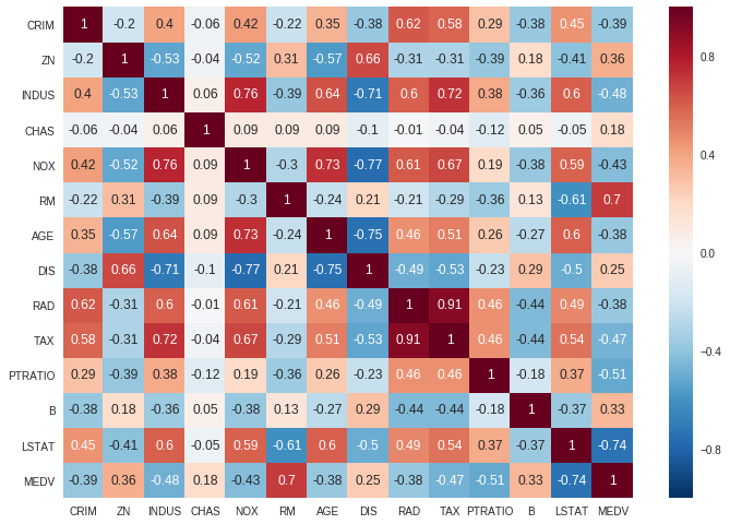
The correlation coefficient ranges from -1 to 1. If the value is close to 1, it means that there is a strong positive correlation between the two features. When it is close to -1, the features have a strong negative correlation.

In the figure above, you can see that the TAX and RAD features have a strong positive correlation and the DIS and NOX features have a strong negative correlation.

If you find out that there are some features in your dataset that are correlated to each other, means that they convey the same information. It is recommended to remove one of them.

You can read more about this here: In supervised learning, why is it bad to have correlated features?

Conclusion

The methods I explained in this article will help you prepare most of the structured datasets you have. But if you are working on unstructured datasets such as images, text, and audio, you will have to learn different methods that are not explained in this article.

The following articles will help you learn how to prepare images or text datasets for your machine learning projects:

Congratulations 👏👏, you have made it to the end of this article! I hope you have learned something new that will help you on your next machine learning or data science project.

If you learned something new or enjoyed reading this article, please share it so that others can see it. Until then, see you in the next post!

You can also find me on Twitter @Davis_McDavid.

And you can read more articles like this here.