
Feature engineering is an essential step in the data preprocessing process, especially when dealing with tabular data.
It involves creating new features (columns), transforming existing ones, and selecting the most relevant attributes to improve the performance and accuracy of machine learning models.
Feature engineering helps the model understand the data’s underlying patterns, relationships, and nuances. It plays a crucial role in the success of a machine learning project, as it can turn a good model into a great one by optimizing the input features. Effective feature engineering also leads to faster training times, and more interpretable results.
Before delving into the realm of feature engineering, you need to recognize the pivotal role of data cleaning in ensuring the success of Feature Engineering. Addressing missing values, handling outliers, and resolving inconsistencies not only improves the integrity of the data but also establishes a solid groundwork for subsequent feature extraction and transformation.
In this tutorial, we'll explore the concept of feature engineering for structured data. We'll cover some techniques such as feature scaling, feature creation, feature selection, and binning. We'll use a hypothetical dataset to demonstrate these various feature engineering techniques.
Let's start by creating some dummy data.
How to Create Dummy Data
We'll use Python and the pandas library to create a dummy dataset for our feature engineering examples. Here's how you can generate dummy data:
import pandas as pd
import numpy as np
# Create a sample dataframe
data = {
'Age': [25, 30, 35, 40, 45],
'Income': [50000, 60000, 75000, 90000, 80000],
'Education': ['High School', 'Bachelor', 'Master', 'Ph.D.', 'Bachelor'],
'City': ['New York', 'San Francisco', 'Chicago', 'Los Angeles', 'Miami'],
'Gender': ['Male', 'Female', 'Male', 'Female', 'Male'],
'Productivity': [5, 4, 3, 2, 4]
}
df = pd.DataFrame(data)
 Code Output
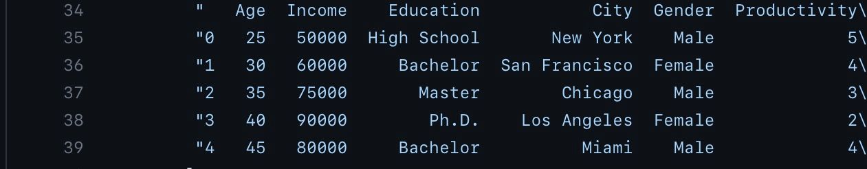
As seen above, the dummy dataset created consists of six features: 'Age,' 'Income,' 'Education,' 'City,' 'Gender,' and 'Productivity.'
Now, let's explore different feature engineering techniques.
One-Hot Encoding
One-hot encoding is a method used to convert categorical variables into a binary matrix. Our dataset has some columns filled with words such as gender, education, and cities.
But machines like numbers, not words. So we’ll use a technique called one-hot encoding. It’s like giving each category its own switch – either it’s on (1) or off (0). It creates a binary column for each category within a categorical feature.
This technique is essential because many machine learning algorithms cannot work directly with categorical data.
One-Hot Encoding Example
Let's apply one-hot encoding to the 'Education' , 'City' and 'Gender' columns in our dataset. We'll use the get_dummies function from pandas for this purpose:
## Perform one-hot encoding
df_encoded = pd.get_dummies(df, columns=['Education', 'City', 'Gender'])
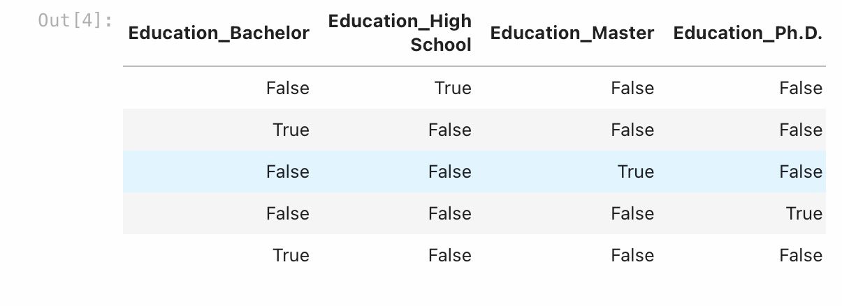
After one-hot encoding, our dataset will now have binary columns for each category within 'Education' 'City' and 'Gender'. This transformation allows machine learning models to understand and utilize these categorical variables effectively.
 Code Output
As you can see in the image above, the categorical columns are now being transformed into a binary matrix.
Feature Scaling
Feature scaling is crucial when working with numerical features that have different scales. Scaling ensures that all features contribute equally to the model, preventing any one feature from dominating the others.
In our data, ‘Age’ and ‘Income’ might have different scales. ‘Age’ might go from 0 to 100, while ‘Income’ could go from 20,000 to 200,000. Feature scaling makes them play nicely together by putting them on the same scale.
Feature Scaling Example
In our dataset, 'Age' and 'Income' have different scales. To scale these features, we'll use the StandardScaler from the sklearn.preprocessing module:
from sklearn.preprocessing import StandardScaler
# Initialize the StandardScaler
scaler = StandardScaler()
# Fit and transform the selected columns
df_encoded[['Age', 'Income']] = scaler.fit_transform(df_encoded[['Age', 'Income']])
 Code Output
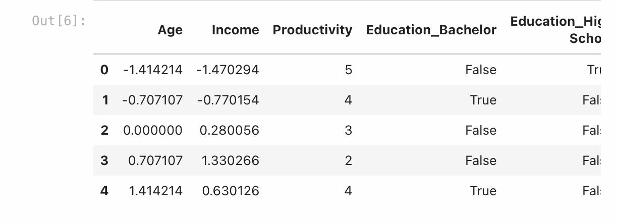
From the code output above, now we can see that the 'Age' and 'Income' have been scaled to have a mean of 0 and a standard deviation of 1. This makes them compatible for modeling and helps algorithms that rely on distances or gradients perform better.
Feature Creation
Feature creation is one of the most pivotal techniques in Feature Engineering. It involves generating new features (columns) from existing ones to provide additional information to the model. It can help uncover complex relationships and patterns within the data.
Let’s say we mix ‘Age’ and ‘Income’ to create a new feature called ‘Income per Age’. This new feature might help our model understand how money and age are related.
Feature Creation Example
In our dataset, we can create a new feature, 'Income per Age,' to capture the relationship between income and age. This can be a useful feature for certain prediction tasks:
# Create a new feature 'Income per Age'
df_encoded['Income per Age'] = df_encoded['Income'] / df_encoded['Age']
 Code Output
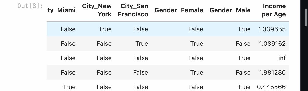
The 'Income per Age' feature provides a measure of income relative to age, which could be valuable in various modeling scenarios. With this an additional column has been created.
Feature Selection
Feature selection is the process of choosing the most relevant features for a given modeling task. Reducing the number of features can improve model performance, reduce overfitting, and speed up training. It makes your model’s job easier because it doesn’t have to deal with unnecessary things.
Feature Selection Example
Let's assume we want to select the most relevant features for predicting 'Productivity.' We can use feature selection techniques like Recursive Feature Elimination (RFE) with a linear regression model:
from sklearn.feature_selection import RFE
from sklearn.linear_model import LinearRegression
# Separate the target variable and the features
X = df_encoded.drop('Productivity', axis=1)
y = df_encoded['Productivity']
# Initialize the linear regression model
model = LinearRegression()
# Perform RFE with cross-validation
rfe = RFE(model, n_features_to_select=3) # Select the top 3 features
fit = rfe.fit(X, y) # Corrected: use X instead of x
# Print the selected features
selected_features = X.columns[fit.support_]
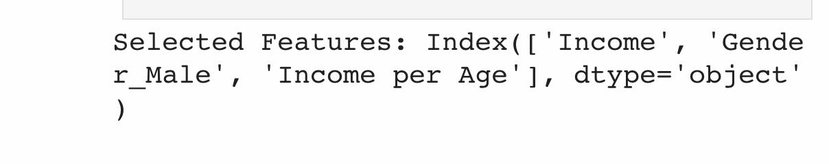
print('Selected Features:', selected_features)
From our data, we used RFE to select the top 3 features that are most relevant for predicting 'Productivity.' This reduces the dimensionality of the data and can improve model performance.
 Code Output
This output received indicates that, according to the Recursive Feature Elimination (RFE) process, the columns: 'Income', 'City_Miami', and 'Gender_Male' are considered the most important or informative for predicting the target variable 'Productivity' using a linear regression model.
Let's break down the interpretation:
- Income: The 'Income' feature is likely identified as an important predictor. It suggests that, according to the RFE process, changes in income have a significant impact on predicting 'Productivity' based on the given linear regression model.
- City_Miami: The presence of 'City_Miami' as an important feature suggests that, in the context of our data, whether an individual is from Miami or not contributes significantly to predicting 'Productivity.'
- Gender_Male: Similarly, the 'Gender_Male' feature is considered important. This implies that, according to the model, the gender of an individual, specifically being male, is informative for predicting 'Productivity.'
It's important to note that the interpretation of "importance" here is specific to the linear regression model used in combination with the RFE feature selection technique. RFE ranks features based on their contribution to the model's performance in predicting the target variable.
Binning and Bucketing
Binning or bucketing involves grouping continuous numerical data into discrete intervals. It can help capture non-linear relationships and make modeling more robust.
Let’s consider a practical example. Based on our dummy data, Instead of treating the "Age" column as a continuous variable, you decide to bin it into categories like "Young," "Mid-career," and "Senior" to better understand how age relates to productivity.
After your analysis, you might discover that employees in the "Mid-career" category tend to have the highest productivity levels. This doesn't mean that age directly causes productivity, but it suggests a potential relationship that could be influenced by factors such as experience, skill development, and familiarity with the job.
By binning age into categories, you've made the age-productivity relationship more interpretable, which can provide your model with more detailed information.
Binning Example
Let's say we want to create bins for the 'Age' feature. We can use the cut function from pandas to define bin boundaries:
# Create bins and labels for the single column
bins = [-float('inf'), -0.5, 0.5, float('inf')] # Adjust the bin edges as needed
labels = ['Young', 'Mid_Career', 'Senior']
# Bin the Age column
df_encoded['Binned_Column'] = pd.cut(df_encoded['Age'], bins=bins, labels=labels, right=False)
# Print the updated DataFrame
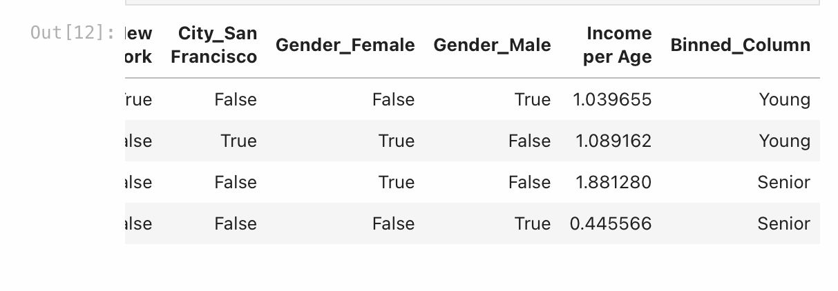
df_encoded
Binning 'Age' into discrete intervals allows the model to consider the age groups as a categorical feature, capturing non-linear relationships.
 Code Output
As you can see above, the 'Age' column has been transformed into a binned column, which further enhances the information given to the model.
Conclusion
Feature engineering techniques enables data scientists and machine learning practitioners to create more informative and relevant features for modeling.
In this tutorial, we explored various feature engineering techniques, including one-hot encoding, feature scaling, feature creation, feature selection, and binning.
Experiment with these techniques to enhance your data analysis and modeling capabilities. Remember that the choice of feature engineering techniques should be driven by the specific requirements of your project and the nature of your data.