

In this article we'll build a dashboard inspired by the recipes in Zelda: Breath of the Wild.
Our dashboard will have multiple data validation dropdown selections for us to choose ingredients. By using a =Query() function, we'll then display the recipes that contain any combination of the selected ingredients.
Let's go!
 gif of man saying, "here we go!"
Final Product
Here's what the finished dashboard will look like. It's not overly complicated, and the tools and techniques we'll use to get the data, clean it, and display it dynamically are quite valuable.
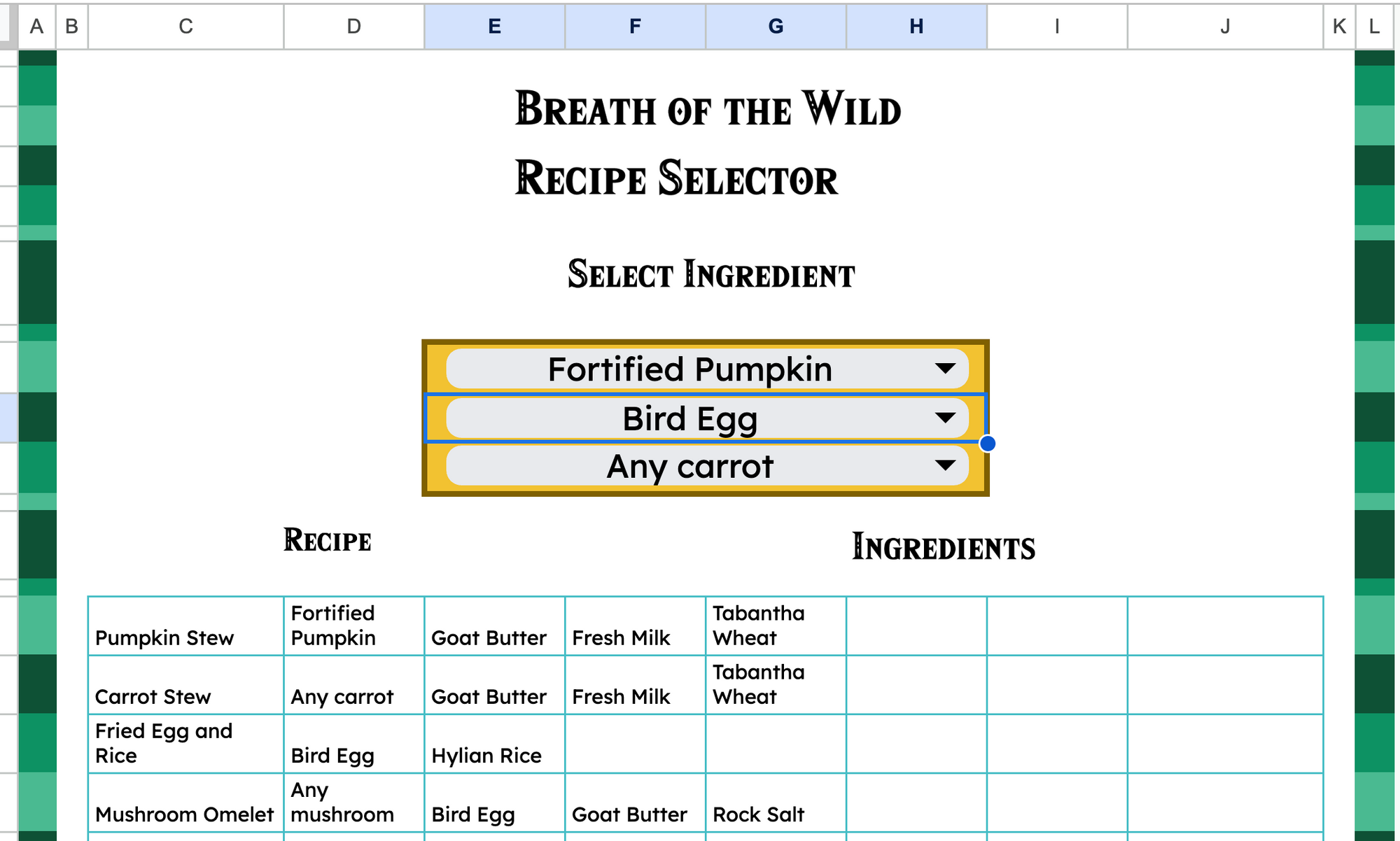 picture of the Zelda dashboard
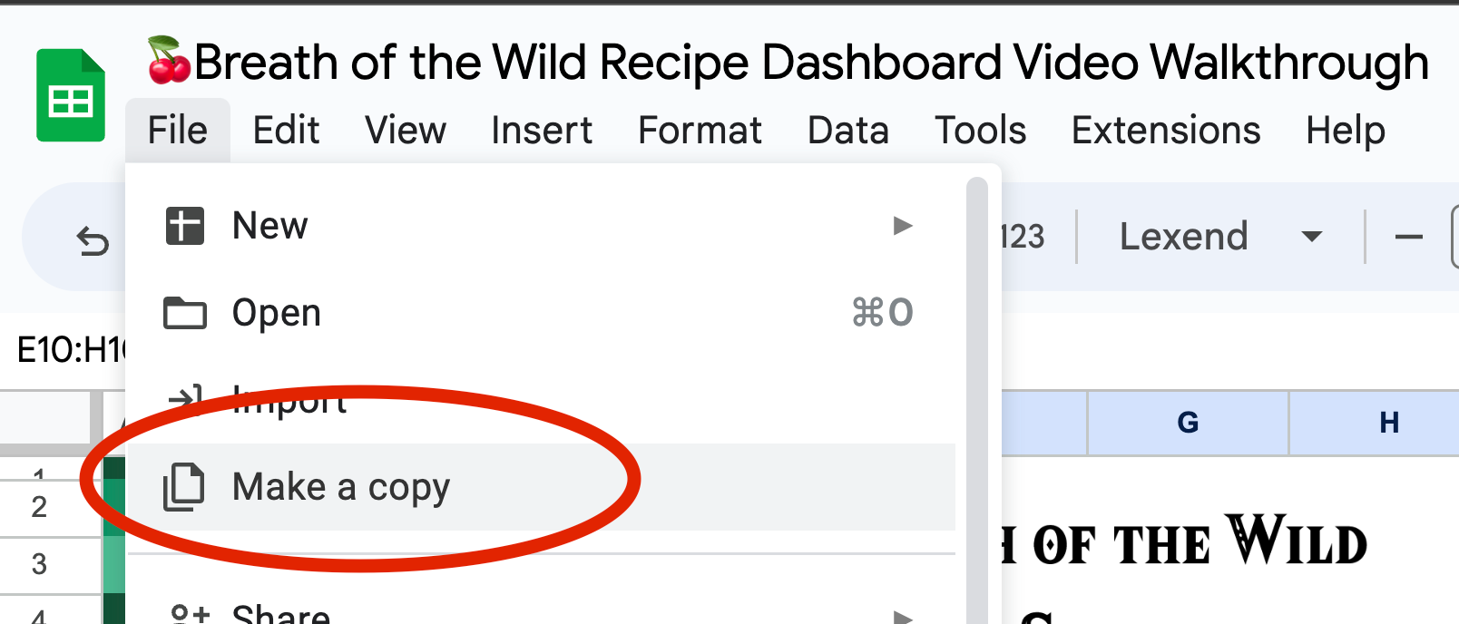
Here's the source code Google Sheet. Open this up to follow along and double check some of the code as you go through the article
You can make an editable copy of this by selecting File -> Make a Copy.
Walkthrough Video
If you'd like to see a video of me building this from scratch, here is a time-lapse 14min video with me narrating the steps:
Project Setup
The first thing we need is data. In our case, we're going to use the IMPORTHTML() function to get data from IGN. IMPORTHTML() allows us to reference a URL, specify whether to search the URL for "tables" or "lists", and then by providing an index number, import the table or list from the URL.
 screenshot of importhtml docs
IGN has a handy recipe cookbook here.
We'll place the URL in a cell in our Google Sheet because after inspecting the page, we see that the recipes are contained within several tables, so we'll need to use multiple import statements.
I've put the URL in D3 and we're ready to import all the tables. In order to do this in one fell swoop, we can use curly brackets. In Google Sheets, curly brackets create arrays.
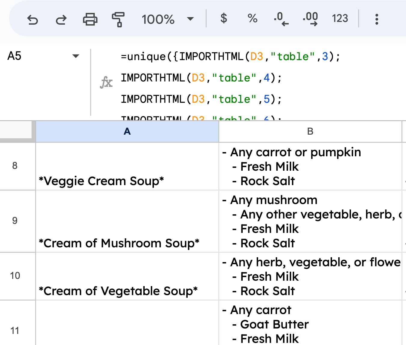
By wrapping multiple IMPORTHTML() statements in curly brackets, we create an array of all those imports. As a final touch, we can wrap the whole thing in a UNIQUE() function to ensure that no duplicate recipes (or in our case, table headers) are brought over to our data tab.
Here's the code:
```google sheets =UNIQUE({IMPORTHTML(D3,"table",3); IMPORTHTML(D3,"table",4); IMPORTHTML(D3,"table",5); IMPORTHTML(D3,"table",6); IMPORTHTML(D3,"table",7); IMPORTHTML(D3,"table",8); IMPORTHTML(D3,"table",9)})
This gives us the data, but we need to clean it up. Specifically, we need to get rid of the asterisks in the meal titles and the dashes, extras spaces, and line breaks in the ingredient lists.
_picture of uncleaned imported data_
## How to Clean the Data
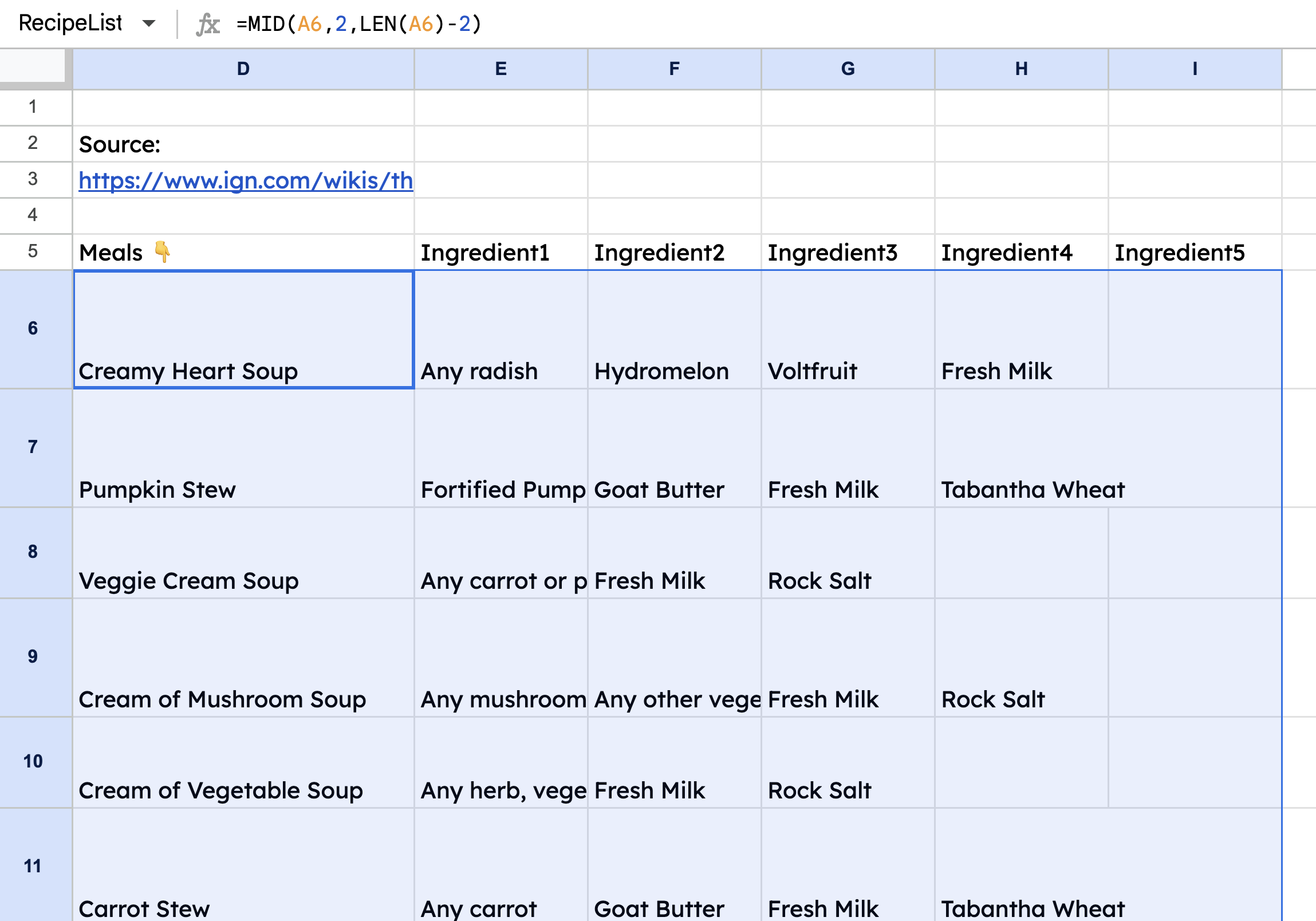
For the titles, we'll use the `MID()` and `LEN()` functions.
```google sheets
//For first row of Meal Titles
=MID(A6,2,LEN(A6)-2)
MID() returns a section of the cell's contents starting at one index and ending at another. We want to grab the contents after the first asterisk, so we'll use 2 as the first index. And then we'll use LEN()-2 to find the length of the cell's contents minus 2 for the ending index.
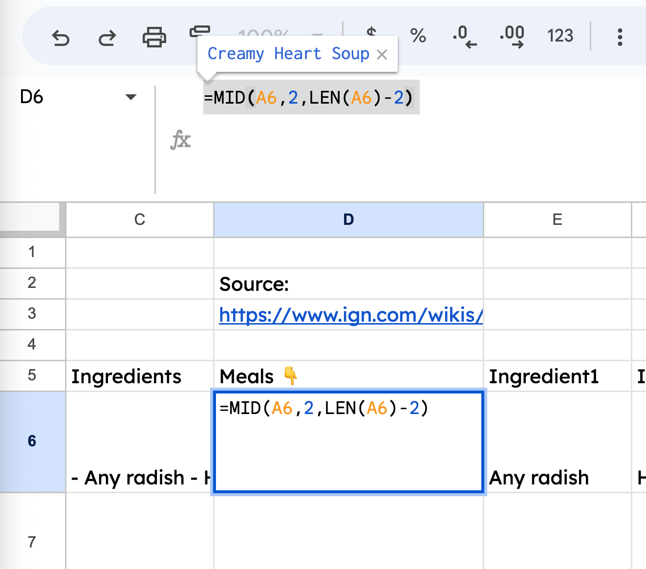 Screenshot of cleaning data in Google Sheet
For the ingredients, we'll first use TRIM(CLEAN()) to remove non-printable characters and extra spaces. Then, we'll use ARRAYFORMULA(TRIM(SPLIT())) to get each remaining ingredient into its own cell.
```google sheets //For first row of Ingredients =ARRAYFORMULA(TRIM(SPLIT(C6,"-")))
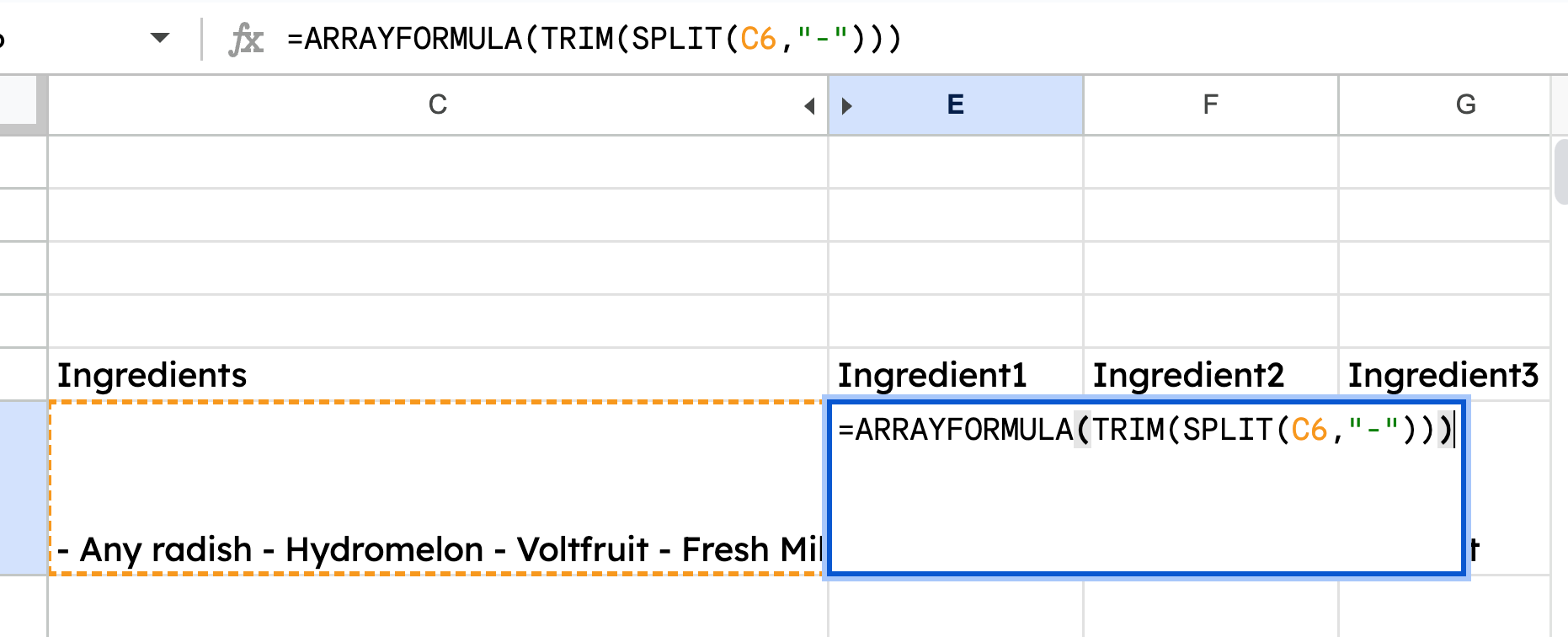
_Screenshot of TRIM, SPLIT and ARRAY FORMULA_
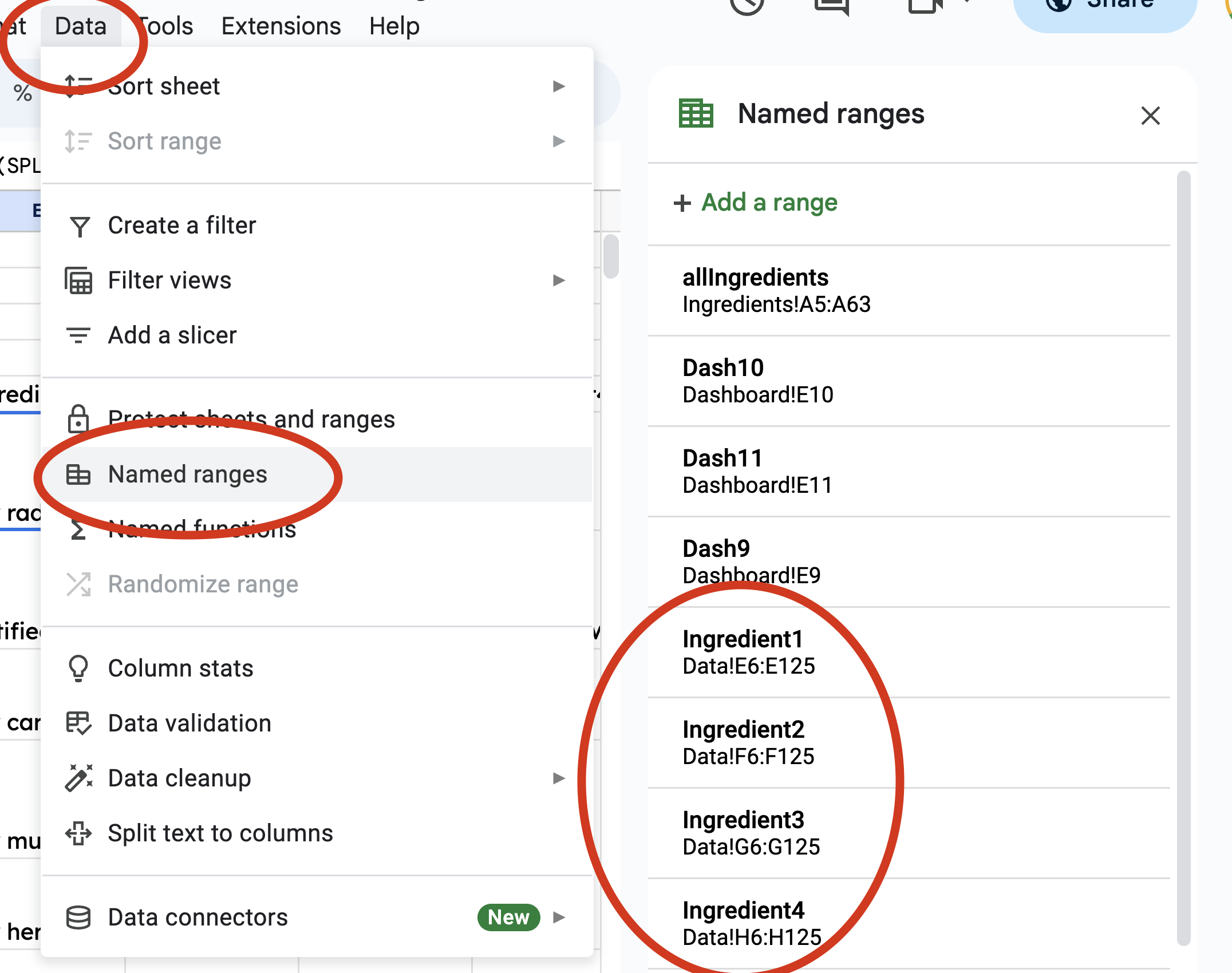
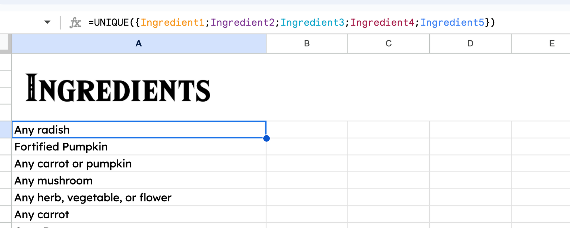
Now that we have our ingredients split into separate cells, let's name some ranges. This will make life easier as we build the dashboard in a moment. 😀
Selecting each column of the ingredients, go to `Data -> named ranges` and name them `Ingredient1`, `Ingredient2`, `Ingredient3`, `Ingredient4`, and `Ingredient5`.
_screenshot of named ranges menu_
Also, select the entire cleaned data range: our meal titles and our individual ingredient columns, and name this range `RecipeList`.
_Screenshot of cleaned full recipe list_
## How to Get All Unique Ingredients
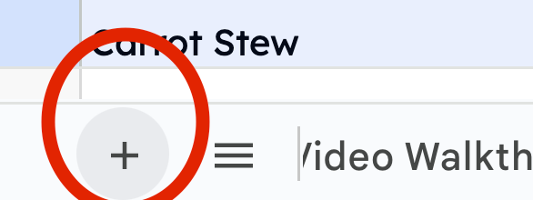
Create a new sheet by clicking the `+` button at the bottom left of the window and name this sheet `Ingredients`.
_Screenshot of add new sheet button_
We now need all the unique ingredients pulled out into a range which we'll name `allIngredients`.
To do this, we'll use the `UNIQUE()` function and all the ingredient named ranges wrapped in curly brackets.
```appscript
=UNIQUE({Ingredient1;
Ingredient2;
Ingredient3;
Ingredient4;
Ingredient5})
This gives us a unique list of ingredients that we'll use as we build the dropdown menus in our dashboard.
How to Make the Dashboard
Create another new sheet and name it Dashboard. Here's where the fun begins. 🔥
 gif of woman saying, fun will now commence.
The first thing we need are some dropdown menus containing all the possible ingredients.
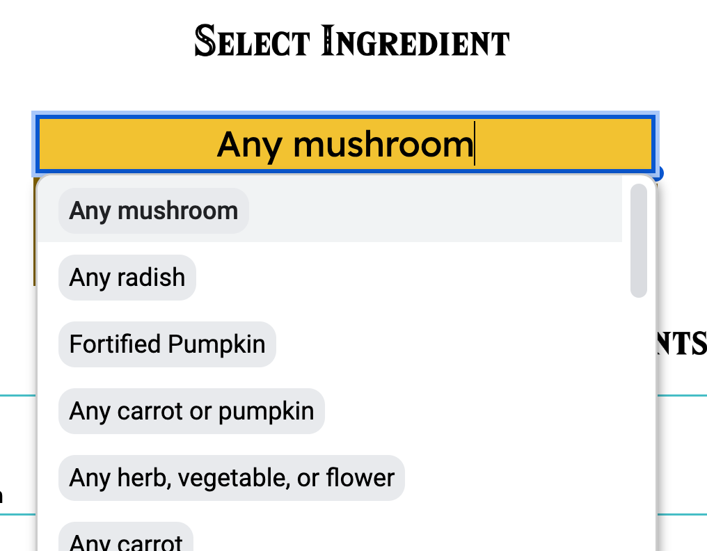 screenshot of dropdown menu
You may either right click in a cell and select Dropdown, or select Data -> Data validation from the Toolbar.
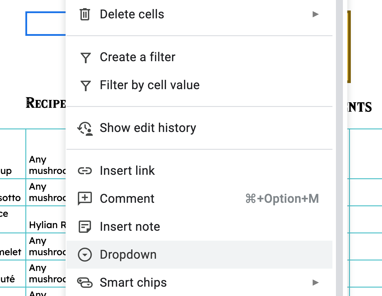 Screenshot of Dropdown option in Google Sheets
Under criteria, select Dropdown (from a range). And in the range, we can input the named range we just created from our Ingredients sheet: =allIngredients.
This will populate all the ingredients beneath the selection. If you'd like, you can even customize the color and appearance options for these. Since there are so many, I left them as default.
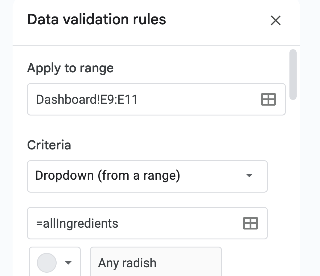 Screenshot of data validation rules.
Simply copy and paste this cell two more times and we have our three identical dropdown menus.
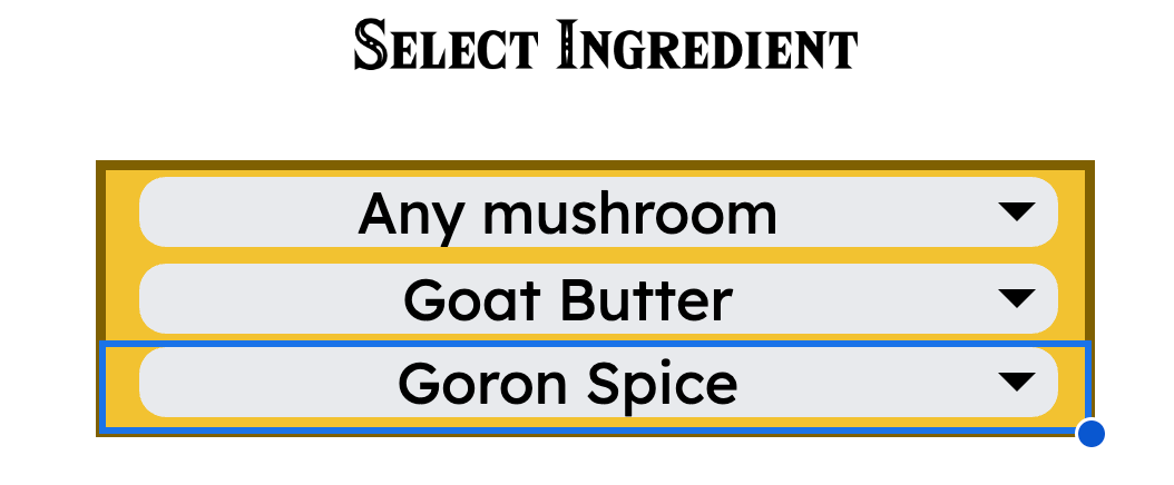 Screenshot of 3 dropdown menus
Logic
We want to handle a few different cases in our dashboard. For any selected ingredient or combination of ingredients, we want to query our RecipeList named range for those ingredients and return the full corresponding recipe.
There are eight possible combinations for the dropdown menus being filled out:
- none
- all
- only the first
- only the second
- only the third
- first and second
- first and third
- second and third.
We need to feed a query statement with different values depending on which of the above states is true.
Let's make another new sheet and name it Formula to spell out and keep track of this logic.
We need a simple test for TRUE or FALSE for each of the possibilities. And to do this, we'll simply test whether or not each of the dropdown menus are blank or contain text.
Conveniently, Google Sheets has two functions that do exactly that: ISBLANK() and ISTEXT().
We'll do some more range naming to make things more legible and then test for each condition.
I've named the three dropdown menu ranges on the Dashboard Dash9, Dash10 and Dash11.
Here's the code to test for when the first and third dropdown menus are filled out:
```google sheets =IF(AND(ISTEXT(Dash9),ISTEXT(Dash10),ISBLANK(Dash11)),true,false)
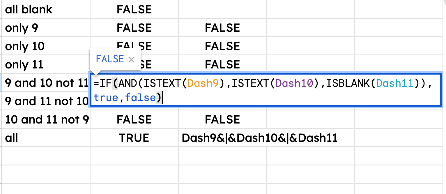
_Screenshot of logic tests_
The `IF` statement returns true or false based on the nested `AND` statement which combines the `ISTEXT` and `ISBLANK` statements for each dropdown menu.
> Stay with me! It's all about to come together! 👊
Now, in order to feed the dropdown menu options to our query statement (which I promise we're about to write!) we need to string it together with bar lines which will function like the `OR` operator in the query.
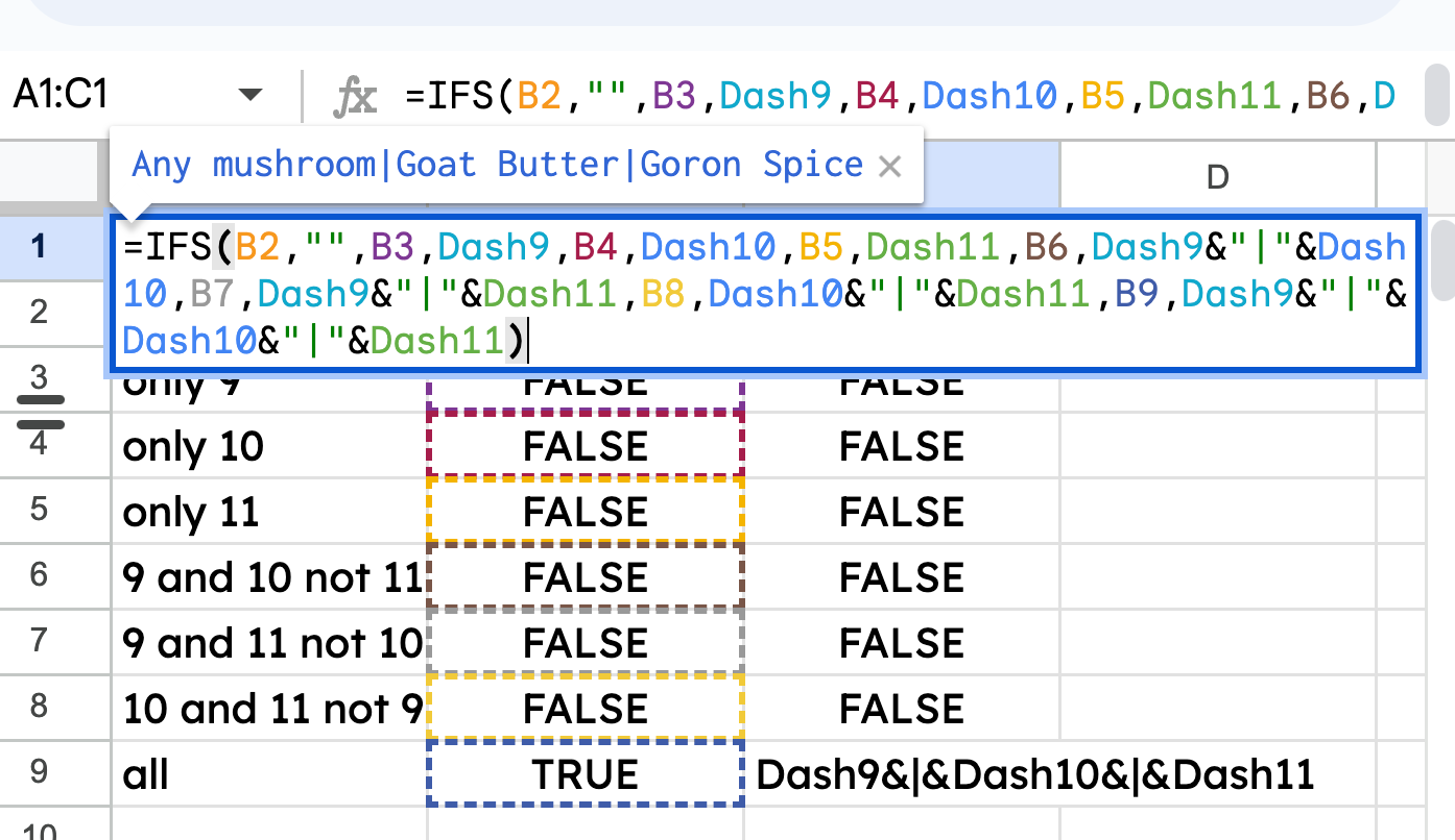
So...in `A1` of our `Formula` sheet, we'll use an `IFS()` function to display the contents of one or more of the `Dash9`, `Dash10` and `Dash11` ranges.
To achieve this when there are more than one with values, we use the `&` operator which concatenates the value in the `Dash` cell with a bar line within quotes ("|"). And the result is shown below.
```google sheets
=IFS(B2,"",
B3,Dash9,
B4,Dash10,
B5,Dash11,
B6,Dash9&"|"&Dash10,
B7,Dash9&"|"&Dash11,
B8,Dash10&"|"&Dash11,
B9,Dash9&"|"&Dash10&"|"&Dash11)
We have our query value built. And it will change dynamically depending on which dropdown menus contain text.
 Screenshot of IFS Statement
Query Statement
Now, the hard work is done. Let's plug what we've created into a query statement on the Dashboard to make this all work!
Query will look at a range, in our case the RecipeList named range with all our meal names and ingredients, and return everything that matches the criteria we feed it.
We want to return a full recipe when our Query named range is matched to an ingredient in any of the five ingredient named ranges.
Here's the full code, and I'll explain it below.
google sheets
=if(Query="","",
QUERY(RecipeList,
"Select *
WHERE E matches'"&Query&"'
OR F matches '"&Query&"'
OR G matches '"&Query&"'
OR H matches '"&Query&"'
OR I matches '"&Query&"'"))
First, if our Query is an empty string, we want nothing to be returned...this is when none of the dropdowns are filled in and the result will be an empty table on the dashboard.
Select *: this means to select all, or return all the values in the query range.
WHERE E matches '"&Query&"': This is the beginning of the criteria. E is literally column E from our Data sheet. That's where the Ingredient1 named range lives. F is where Ingredient2 is...and so on.
By using matches, we are telling the query to see if any value in the Query named range matches any value in each of the specified ingredient columns. We have to use the funky syntax of single and double quotes to make the query function know that we're using that Query named range and not the word or string, "Query".
The bar lines in our Query named range functions as the OR operator, so when there are multiple ingredients in the dropdown list, the query statement looks in each column for either one or the other ingredient.
Conclusion
This was a ton of fun to make, and I hope you've been able to learn some valuable skills by following along.
We've imported data, cleaned it up, created named ranges, dropdown menus and dynamically changing logical tests...all for the sake of a query statement that returns the recipes we need based on the ingredient(s) we give it.
Come follow me on YouTube where I'm making more content like this weekly. 👋
Have a great one!