

What is the Gradient Descent Algorithm?
Gradient descent is probably the most popular machine learning algorithm. At its core, the algorithm exists to minimize errors as much as possible.
The aim of gradient descent as an algorithm is to minimize the cost function of a model. We can tell this from the meanings of the words ‘Gradient’ and ‘Descent’.
While gradient means the gap between two defined points (that is the cost function in this context), descent refers to downward motion in general (that is minimizing the cost function in this context).
So in the context of machine learning, Gradient Descent refers to the iterative attempt to minimize the prediction error of a machine learning model by adjusting its parameters to yield the smallest possible error.
This error is known as the Cost Function. The cost function is a plot of the answer of the question “by how much does the predicted value differ from the actual value?”. While the way to evaluate cost functions often differs for different machine learning models, in a simple linear regression model, it is usually the root mean squared error of the model.
 A 3D plot of the cost function of a simple linear regression model with M representing the minimum point
It is important to note that for the simpler models like the linear regression, a plot of the cost function is usually bow-shaped, which makes it easier to ascertain the minimum point. However, this is not always the case. For more complex models (for instance neural networks), the plot might not be bow-shaped. It is possible for the cost function to have multiple minimum points as shown in the image below.
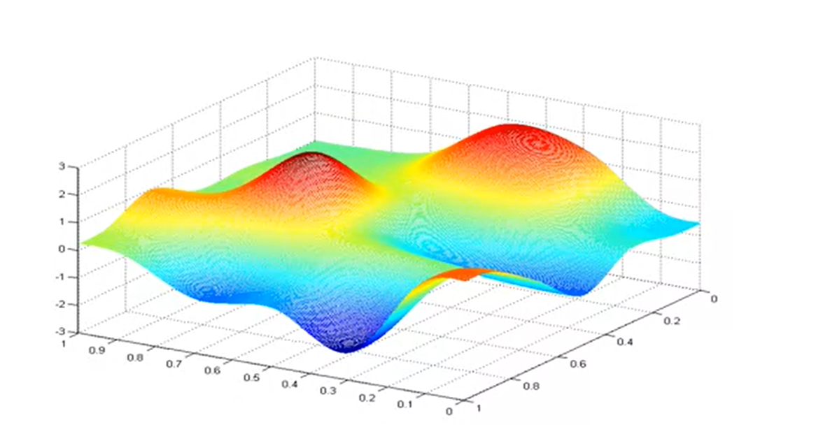 A 3D plot of the cost function of a neural network. Source: Coursera
How Does Gradient Descent Work?
Firstly, it is important to note that like most machine learning processes, the gradient descent algorithm is an iterative process.
Assuming you have the cost function for a simple linear regression model as j(w,b) where j is a function of w and b, the gradient descent algorithm works such that it starts off with some initial random guess for w and b. The algorithm will keep tweaking the parameters w and b in an attempt to optimize the cost function, j.
In linear regression, the choice for the initial values does not matter much. A common choice is zero.
The perfect analogy for the gradient descent algorithm that minimizes the cost-function j(w, b) and reaches its local minimum by adjusting the parameters w and b is hiking down to the bottom of a mountain or hill (as shown in the 3D plot of the cost function of a simple linear regression model shown earlier). Or, trying to get to the lowest point of a golf course. In either case, they will make repetitive short steps till they make it to the bottom of the mountain or hill.
The Gradient Descent Formula
Here's the formula for gradient descent: b = a - γ Δ f(a)
The equation above describes what the gradient descent algorithm does.
That is b is the next position of the hiker while a represents the current position. The minus sign is for the minimization part of the gradient descent algorithm since the goal is to minimize the error as much as possible. γ in the middle is a factor known as the learning rate, and the term Δf(a) is a gradient term that defines the direction of the minimum point.
As such, this formula tells the next position for the hiker/the person on the golf course (that is the direction of the steepest descent). It is important to note that the term γΔ f(a) is subtracted from a because the goal is to move against the gradient, toward the local minimum.
What is the Learning Rate?
The learning rate is the determinant of how big the steps gradient descent takes in the direction of the local minimum. It determines the speed with which the algorithm moves towards the optimum values of the cost function.
Because of this, the choice of the learning rate, γ, is important and has a significant impact on the effectiveness of the algorithm.
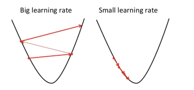
If the learning rate is too big as shown above, in a bid to find the optimal point, it moves from the point on the left all the way to the point on the right. In that case, you see that the cost function has gotten worse.
On the other hand, if the learning rate is too small, then gradient descents will work, albeit very slowly.
It is important to pick the learning rate carefully.
How to Implement Gradient Descent in Linear Regression
import numpy as np
import matplotlib.pyplot as plt

class Linear_Regression:
    def __init__(self, X, Y):
        self.X = X
        self.Y = Y
        self.b = [0, 0]

    def update_coeffs(self, learning_rate):
        Y_pred = self.predict()
        Y = self.Y
        m = len(Y)
        self.b[0] = self.b[0] - (learning_rate * ((1/m) * np.sum(Y_pred - Y)))
        self.b[1] = self.b[1] - (learning_rate * ((1/m) * np.sum((Y_pred - Y) * self.X)))

    def predict(self, X=[]):
        Y_pred = np.array([])
        if not X: X = self.X
        b = self.b
        for x in X:
            Y_pred = np.append(Y_pred, b[0] + (b[1] * x))

        return Y_pred

    def get_current_accuracy(self, Y_pred):
        p, e = Y_pred, self.Y
        n = len(Y_pred)
        return 1-sum(
            [
                abs(p[i]-e[i])/e[i]
                for i in range(n)
                if e[i] != 0]
        )/n
    #def predict(self, b, yi):

    def compute_cost(self, Y_pred):
        m = len(self.Y)
        J = (1 / 2*m) * (np.sum(Y_pred - self.Y)**2)
        return J

    def plot_best_fit(self, Y_pred, fig):
                f = plt.figure(fig)
                plt.scatter(self.X, self.Y, color='b')
                plt.plot(self.X, Y_pred, color='g')
                f.show()


def main():
    X = np.array([i for i in range(11)])
    Y = np.array([2*i for i in range(11)])

    regressor = Linear_Regression(X, Y)

    iterations = 0
    steps = 100
    learning_rate = 0.01
    costs = []

    #original best-fit line
    Y_pred = regressor.predict()
    regressor.plot_best_fit(Y_pred, 'Initial Best Fit Line')


    while 1:
        Y_pred = regressor.predict()
        cost = regressor.compute_cost(Y_pred)
        costs.append(cost)
        regressor.update_coeffs(learning_rate)

        iterations += 1
        if iterations % steps == 0:
            print(iterations, "epochs elapsed")
            print("Current accuracy is :",
                regressor.get_current_accuracy(Y_pred))

            stop = input("Do you want to stop (y/*)??")
            if stop == "y":
                break

    #final best-fit line
    regressor.plot_best_fit(Y_pred, 'Final Best Fit Line')

    #plot to verify cost function decreases
    h = plt.figure('Verification')
    plt.plot(range(iterations), costs, color='b')
    h.show()

    # if user wants to predict using the regressor:
    regressor.predict([i for i in range(10)])

if __name__ == '__main__':
    main()
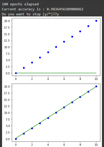
At its core, you can see that the block of code trains a gradient descent algorithm for a linear regression machine learning model using 0.01 as its learning rate on 100 steps.
Upon running the code above, the output shown is given below:

Conclusion
In conclusion, it is important to note that the gradient descent algorithm is especially important in the artificial intelligence and machine learning domains as the models must be optimized for accuracy.
In this article, you learnt what the Gradient Descent algorithm is, how it works, its formula, what learning rate is, and the importance of picking the right learning rate. You also saw a code illustration of how Gradient Descent works.
Finally, I share my writings on Artificial Intelligence, Machine Learning and Microsoft Azure on Twitter if you enjoyed this article and want to see more.